PicoScope 9400 Series

5 or 16 GHz bandwidth
4 channels
500 MSa/s RT sampling rate
Up to 16 GHz trigger

The PicoScope 9400 Series is a new class of SXRTO oscilloscopes that combine the benefits of real-time sampling, equivalent-time sampling and high analog bandwidth.

5 & 16 GHz Sampler Extended Real Time Oscilloscopes

The PicoScope 9400 Series is a new class of SXRTO oscilloscopes that combine the benefits of real-time sampling, equivalent-time sampling and high analog bandwidth.


  • SXRTO (sampler-extended real-time oscilloscope)
  • 9404-16: 16 GHz bandwidth, 22 ps transition time and 2.5 TS/s (0.4 ps resolution) equivalent-time sampling
  • 9404-05: 5 GHz bandwidth, 70 ps transition time and 1 TS/s (1 ps resolution) equivalent-time sampling
  • Pulse, eye and mask testing down to 100 ps and up to 8 Gb/s
  • Four 12-bit 500 MS/s ADCs
  • Intuitive and configurable touch-compatible Windows user interface
  • Comprehensive built-in measurements, zooms, data masks and histograms
  • ±800 mV full-scale input range into 50 Ω
  • 10 mV/div to 0.25 V/div ranges provided by digital gain
  • Up to 250 kS trace length, shared between channels
  • Optional clock and data recovery (8 Gb/s on 9404-16, 5 Gb/s on 9404-05)
The PicoScope 9400 Series SXRTOs have four input channels up to 16 GHz with market-leading ADC, timing and display resolutions for accurately measuring and visualizing high-speed analog and data signals. They are ideal for capturing pulse and step transitions down to 22 ps, impulses down to 45 ps and clocks and data eyes to 8 Gb/s. Most high-bandwidth applications involve repetitive signals or clock-related data streams that can be readily analyzed by equivalent-time sampling (ETS). The SXRTO quickly builds ETS, persistence displays and statistics. It has a built-in full-bandwidth trigger on every channel, with pretrigger ETS capture to well above the Nyquist sampling rate. There are three acquisition modes—real time, ETS and roll—all capturing at 12-bit resolution into a shared memory of 250 kS.

The PicoSample 4 software is derived from our existing PicoSample 3 and PicoScope 9000 products, which together represent over ten years of development, customer feedback and optimization.

The high-resolution display can be resized to fit any window, filling 4k and even larger monitors or arrays of monitors. Four independent zoom channels can show you different views of your data down to a resolution of 0.4 ps. Most of the controls and status panels can be shown or hidden according to your application, allowing you to make optimal use of the display area.

The oscilloscope has a 2.5 GHz direct trigger that can be driven from any input channel, and a built-in prescaler can extend the trigger bandwidth to 5 GHz. The external prescaler on the 9404-16 extends this further to 16 GHz.

These compact units are small enough to place on your workbench close to the device under test. Now, instead of using remote probe heads attached to a large benchtop unit, all you need is a short, low-loss coaxial cable. Everything else you need is built into the oscilloscope, with no expensive hardware or software add-ons to worry about, and we don’t charge you for new software features and updates.


Typical applications

  • Telecom and radar test, service and manufacturing
  • Optical fiber, transceiver and laser testing (optical to electrical conversion not included)
  • RF, microwave and gigabit digital system measurements
  • Signal, eye, pulse and impulse characterization
  • Precision timing and phase analysis
  • Digital system design and characterization
  • Eye diagram, mask and limits test up to 8 Gb/s
  • Clock and data recovery at up to 8 Gb/s
  • Ethernet, HDMI 1, PCI, SATA, USB 2.0
  • Semiconductor characterization
  • Signal, data and pulse/impulse integrity and pre-compliance testing


High-bandwidth probes

The PicoConnect 900 Series low-impedance, high-bandwidth probes are ideal companions for the PicoScope 9400 Series, allowing cost-effective fingertip browsing of fast signals. Two series are available:

  • RF, microwave and pulse probes for broadband signals up to 5 GHz (10 Gb/s)
  • Gigabit probes for data streams such as USB 2, HDMI 1, Ethernet, PCIe and SATA


Other features

Bandwidth limit filters

A selectable analog bandwidth limiter (100 or 450 MHz) on each input channel can be used to reject high frequencies and associated noise. The narrow setting can be used as an anti-alias filter.


Frequency counter

A dedicated frequency counter shows signal frequency (or period) at all times, regardless of measurement and timebase settings, with a resolution of 1 ppm.


Optional clock and data recovery

Clock and data recovery (CDR) is now available as a factory-fitted optional trigger feature for the PicoScope 9404-16 and 9404-05 SXRTOs.

Associated with high-speed serial data applications, clock and data recovery will already be familiar to PicoScope 9300 users. While low-speed serial data can often be accompanied by a separate clock signal, at high speed this approach would create timing skew and jitter between the clock and the data that could prevent accurate data decoding. Thus high-speed data receivers will generate a new clock, and using a phase-locked loop technique they will lock and align that new clock to the incoming data stream. This is the recovered clock, which can then be used to decode and thus recover data accurately. They have also saved the cost of an entire clock signal path by now needing only the serial data signal.

In many applications requiring our oscilloscopes to view the data, the data generator and its clock will be close at hand and we can trigger off that clock. However, if only the data is available (at the far end of an optical fiber, for instance), we will need the CDR option to recover the clock and then trigger off that instead. We may also need to use the CDR option in demanding eye and jitter measurements. This is because we want our instrument to measure as exactly as possible the signal quality that a recovered clock and data receiver will “see”.

When fitted, the PicoScope 9400 CDR option can be selected as the trigger source from any input channel. Additionally, for use by other instruments or by downstream system elements, two SMA(f) outputs present recovered clock and recovered data from the rear panel.

Contact Pico to order this option.

SXRTO explained

The real-time oscilloscope

Real-time oscilloscopes (RTOs) are designed with a high enough sampling rate to capture a transient, non-repetitive signal with the instrument’s specified analog bandwidth. According to Nyquist’s sampling theorem, for accurate capture and display of the signal the scope’s sampling rate must be at least twice the signal bandwidth. Typical high-bandwidth RTOs exceed this sampling rate by perhaps a factor of two, achieving up to four samples per cycle, or three samples in a minimum-width impulse.


Equivalent-time sampling

For signals close to or above the RTO’s Nyquist limit, many RTOs can switch to a mode called equivalent-time sampling (ETS). In this mode the scope collects as many samples as it can for each of many trigger events, each trigger contributing more and more samples and detail in a reconstructed waveform. Critical to alignment of these samples is a separate and precise measurement of time between each trigger and the next occurring sample clock.

After a large number of trigger events the scope has enough samples to display the waveform with the desired time resolution. This is called the effective sampling resolution (the inverse of the effective sampling rate), which is many times higher than is possible in real-time (non-ETS) mode.

As this technique relies on a random relationship between trigger events and the sampling clock, it is more correctly called random equivalent-time sampling (or sometimes random interleaved sampling, RIS). It can only be used for repetitive signals – those that vary little from one trigger event to the next.


The sampler-extended real-time oscilloscope (SXRTO)

The PicoScope 9404-16 maximum effective sampling rate in ETS is 2.5 TS/s, with a timing resolution of 0.4 ps, which is 10 000 times higher than the scope’s actual sampling rate.

With an analog bandwidth of up to 16 GHz, the PicoScope 9404-16 SXRTO would require a sampling rate exceeeding 32 GS/s to meet Nyquist’s criterion and somewhat more than this (perhaps 80 GS/s) to reveal wave and pulse shapes. Using ETS, the 9404-16 gives us 156 sample points in a single cycle or a generous 55 samples between 10% and 90% of its fastest transition time.


So is the SXRTO a sampling scope?

All this talk of sampling rates and sampling modes may suggest that the SXRTO is a type of sampling scope, but this is not the case. The name sampling scope, by convention, refers to a different kind of instrument. A sampling scope uses a programmable delay generator to take samples at regular intervals after each trigger event. The technique is called sequential equivalent-time sampling and is the principle behind the PicoScope 9300 Series sampling scopes. These scopes can achieve very high effective sampling rates but have two main drawbacks: they cannot capture data before the trigger event, and they require a separate trigger signal – either from an external source or from a built-in clock-recovery module.

We’ve compiled a table to show the differences between the types of scopes mentioned on this page. The example products are all compact, 4-channel, USB PicoScopes.


Real-time scope SXRTO Sampling scope
Model PicoScope 6407 PicoScope 9400 Series PicoScope 9300 Series
Analog bandwidth 1 GHz* Upto 16 GHz Up to 25 GHz
Real-time sampling 5 GS/s 500 MS/s 1 MS/s
Sequential equivalent-time sampling No No 15 TS/s
Random equivalent-time sampling 200 GS/s Up to 2.5 TS/s 250 MS/s
Trigger on input channel Yes Yes Yes,  but only to 100 MHz bandwidth – requires external trigger or internal clock recovery option.
Pretrigger capture Yes Yes No**
Vertical resolution 8 bits 12 bits 16 bits
Cost (2019 prices) $10k $19.5k $22k

PicoScope 9400 Series – Software

Designed for ease of use

The PicoSample 4 workspace takes full advantage of your screen or array of screens, allowing you to resize the window to fit any display resolution supported by Windows.


On very high-resolution displays, PicoSample 4 plots more samples to give you an even more detailed view of your data.

You decide how much space to give to the trace display and the measurements display, and whether to open or hide the control menus. The user interface is fully touch- or mouse-operable, with grabbing and dragging of traces, cursors, regions and parameters. In touchscreen mode, an enlarged parameter control is displayed to assist adjustments on smaller touchscreen displays.

To zoom, either draw a zoom window or use the numerical zoom and offset controls. You can display up to four different zoomed views of the displayed waveforms.

“Hidden trace” icons show a live view of any channels that are not visible on the main display.

The interaction of timebase, sampling rate and capture size is normally handled automatically, but there is also an option to override this and specify the relative priorities of these three parameters.


A choice of screen formats

When working with multiple traces, you can display them all on one grid or separate them into two or four grids. You can also plot signals in XY mode with or without additional voltage-time grids. The persistence display modes use color-contouring or shading to show statistical variations in the signal. Trace display can be in either dots-only or vector format and all these display settings can be independent, trace by trace. Custom trace labeling is also available.

Measurements

Waveform measurements with statistics

Waveform parameters can be measured in both X and Y axes including X period, frequency, negative or positive cross and jitter. In the Y axis measurements such as max, min, DC RMS and cycle mean are available. Measurements can be within a single trace or trace-to-trace such as phase, delay and gain.

Selection of a measurement parameter displays its values, thresholds and bounds on the main display


Eye diagram measurements

The PicoScope 9400 Series scopes quickly measure more than 70 fundamental parameters used to characterize non‑return‑to‑zero (NRZ) signals and return-to-zero (RZ)
signals.

Up to ten parameters can be measured simultaneously, with comprehensive statistics also shown. The parameters include X-axis measurements such as bit rate and jitter, and Y-axis measurements such as eye height and noise.

Mask testing

PicoSample 4 has a built-in library of over 130 masks for testing data eyes. It can count or capture mask hits or route them to an alarm or acquisition control. You can stress-test against a mask using a specified margin, and locally compile or edit masks.

There’s a choice of gray-scale and color-graded display modes, and a histogramming feature, all of which aid in analyzing noise and jitter in eye diagrams. There is also a statistical display showing a failure count for both the original mask and the margin.

The extensive menu of built-in test waveforms is invaluable for checking your mask test setup before using it on live signals.

Trending

The Trend function displays the evolution of timing parameters as line graphs whose vertical axes are the value of the parameter, and horizontal axes the order in which the values were acquired. The information obtained from applying timing parameters can then be analyzed using Trend.

The following trend parameters can be used: Period, Frequency, Positive Width, Negative Width, Rise Time, Fall Time, Positive Duty Cycle, Negative Duty Cycle.

Trend effectively measures parameters such as oscilloscope timebase linearity.


Please give us your feedback about PicoScope 9400 Series

Your opinion is very important to us. We appreciate your feedback and will use it to evaluate changes and make improvements in our products:

PicoScope 9400 Series Downloads

Here you can download the latest PicoScope 9400 Series Data Sheets, Manuals, Guides and other relevant documents:

PicoScope 9400 Series – Specifications

9404-05 9404-16
Vertical
Number of input channels Four channels. All channels are identical and digitized simultaneously.
*Analog bandwidth (–3 dB)[1] Full: DC to 5 GHz
Middle: DC to 450 MHz
Narrow: DC to 100 MHz
Full: DC to 16 GHz
Middle: DC to 450 MHz
Narrow: DC to 100 MHz
*Passband flatness Full: ±1 dB to 3 GHz Full: ±1 dB to 5 GHz
Calculated rise time (Tr), typical Calculated from the bandwidth.
10% to 90%: calculated from Tr = 0.35/BW
20% to 80%: calculated from Tr = 0.25/BW
Full: 10% to 90%: ≤ 70 ps, 20% to 80%: ≤ 50 ps
Middle: 10% to 90%: ≤ 780 ps, 20% to 80%: ≤ 560 ps
Narrow: 10% to 90%: ≤ 3.5 ns. 20% to 80%: ≤ 2.5 ns
Full: 10% to 90%: ≤ 22 ps, 20% to 80%: ≤ 15.7 ps
Step response, typical Full bandwidth

Overshoot: < 8%
Ringing:
±6% to 3 ns
±4% from 3 ns to 10 ns
±3% from 10 ns to 100 ns
±2% from 100 ns to 400 ns
±1% above 400 ns

Middle bandwidth

Overshoot: < 6%
Ringing:
±4% to 10 ns
±3% from 10 ns to 100 ns
±2% from 100 ns to 400 ns
±1% above 400 ns

Narrow bandwidth

Overshoot: < 5%
Ringing:
±5% to 20 ns
±3% from 20 ns to 100 ns
±2% from 100 ns to 400 ns
±1% above 400 ns

*RMS noise Full: 1.8 mV, maximum, 1.6 mV, typical
Middle: 0.8 mV, maximum, 0.65 mV, typical
Narrow: 0.6 mV, maximum, 0.45 mV, typical
Full: 2.4 mV, maximum, 2.2 mV, typical
Middle: 0.8 mV, maximum, 0.65 mV, typical
Narrow: 0.6 mV, maximum, 0.45 mV, typical
Scale factors (sensitivity) 10 mV/div to 250 mV/div
Full scale is 8 vertical divisions
Adjustable in a 10-12.5-15-20-25-30-40-50-60-80-100-125-150-200-250 mV/div sequence.
Also adjustable in 1% fine increments or better.
With manual or calculator data entry the increment is 0.1 mV/div.
*DC gain accuracy ±2% of full scale. ±1.5% of full scale, typical
Position range ±4 divisions from center screen
DC offset range Adjustable from –1 V to +1 V in 10 mV increments (coarse). Also adjustable in fine increments of 2 mV.
With manual or calculator data entry the increment is 0.01 mV for offset between –99.9 and 99.9 mV, and 0.1 mV for offset between –999.9 and 999.9 mV.
Referenced to the center of display graticule
* Offset accuracy ±2 mV ±2% of offset setting. ±1 mV ±1% of offset setting, typical
Operating input voltage ±800 mV
Vertical zoom and position For all input channels, waveform memories, or functions
Vertical factor: 0.01 to 100
Vertical position: ±800 divisions maximum of zoomed waveform
Channel-to-channel crosstalk (channel isolation) ≥ 50 dB (316:1) for input frequency DC to 1 GHz
≥ 40 dB (100:1) for input frequency > 1 GHz to 3 GHz
≥ 36 dB (63:1) for input frequency > 3 GHz to ≤ 5 GHz
≥ 50 dB (316:1) for input frequency DC to 1 GHz
≥ 40 dB (100:1) for input frequency > 1 GHz to 3 GHz
≥ 36 dB (63:1) for input frequency > 3 GHz to ≤ 16 GHz
Delay between channels ≤ 10 ps, typical
Between any two channels, full bandwidth, equivalent time
ADC resolution 12 bits
Hardware vertical resolution 0.4 mV/LSB without averaging
Overvoltage protection ±1.4 V (DC + peak AC)
* Input impedance (50 ±1.5) Ω. (50 ±1) Ω, typical
Input match Reflections for 70 ps rise time: 10% or less Reflections for 50 ps rise time: 10% or less.
Input coupling DC
Input connectors SMA female
Internal probe power 6.0 W total maximum with PSU as supplied.
Probe power per probe 3.3 V: 100 mA maximum
12 V: 500 mA maximum to total probe power stated above.
Attenuation Attenuation factors may be entered to scale the oscilloscope for external attenuators connected to the channel inputs
Range: 0.0001:1 to 1 000 000:1
Units: Ratio or dB
Scale: Volt, Watt, Ampere, or unknown
9404-05 9404-16
Horizontal
Timebase Internal timebase common to all input channels.
Timebase range Full horizontal scale is 10 divisions
Real time sampling: 10 ns/div to 1000 s/div
Random equivalent time sampling:

50 ps/div to 5 µs/div

20 ps/div to 5 μs/div
Roll: 100 ms/div to 1000 s/div
Segmented: Total number of segments: 2 to 1024. Rearm time between segments: <1 μs (trigger hold-off setting dependent)
Horizontal zoom and position For all input channels, waveform memories, or functions
Horizontal factor: From 1 to 2000
Horizontal position: From 0% to 100% non-zoomed waveform
Timebase clock accuracy Frequency: 500 MHz
Initial set tolerance: ±10 ppm @ 25 °C ±3 °C
* Overall frequency stability: ±50 ppm over operating temperature range
Aging ±7 ppm over 10 years @ 25 °C
Timebase resolution 1.0 ps 0.4 ps
* Delta time measurement accuracy ±(50 ppm * reading + 0.1% * screen width + 5 ps)
Pre-trigger delay Record length ÷ current sampling rate (when delay = 0)
Post-trigger delay 0 to 4.28 s. Coarse increment is one horizontal scale division, fine increment is 0.1 horizontal scale division, manual or calculator increment is 0.01 horizontal scale division.
Channel-to-channel deskew range ±50 ns range. Coarse increment is 100 ps, fine increment is 10 ps. With manual or calculator data entry the increment is four significant digits or 1 ps.
9404-05 9404-16
Acquisition
Sampling modes Real time: Captures all of the sample points used to reconstruct a waveform during a single trigger event
Random equivalent time: Acquires sample points over several trigger events, requiring the input waveform to be repetitive
Roll: Acquisition data will be displayed in a rolling fashion starting from the right side of the display and continuing to the left side of the display (while the acquisition is running)
Maximum sampling rate Real time: 500 MS/s per channel simultaneously
Random equivalent time:

Up to 1 TS/s or 1 ps trigger placement resolution)

Random equivalent time:

Up to 2.5 TS/s or 0.4 ps trigger placement resolution

Record length Real time sampling: From 50 S/ch to 250 kS/ch for one channel, to 125 kS/ch for two channels, to 50 kS/ch for three and four channels
Random equivalent time sampling: From 500 S/ch to 250 kS/ch for one channel, to 125 kS/ch for two channels, to 50 kS/ch for three and four channels
Duration at highest sample rate 0.5 ms for one channel, 0.25 ms for two channels, 0.125 ms for three and four channels
Acquisition modes Sample (normal): Acquires first sample in decimation interval and displays results without further processing
Average: Average value of samples in decimation interval. Number of waveforms for average: 2 to 4096.
Envelope: Envelope of acquired waveforms. Minimum, Maximum or both Minimum and Maximum values acquired over one or more acquisitions. Number of acquisitions is from 2 to 4096 in ×2 sequence and continuously.
Peak detect: Largest and smallest sample in decimation interval. Minimum pulse width: 1/(sampling rate) or 2 ns @ 50 µs/div or faster for single channel.
High resolution: Averages all samples taken during an acquisition interval to create a record point. This average results in a higher-resolution, lower-bandwidth waveform. Resolution can be expanded to 12.5 bits or more, up to 16 bits.
Segmented: Segmented memory optimizes available memory for data streams that have long dead times between activity.
Number of segments: 2 to 1024
Dead time between segments: 3 µs
User can view selected segment, overlaid segments or selected plus overlay.
Search segments: step through, gated block and binary search. Segments are delta and absolute time stamped.
9404-05 9404-16
Trigger
Trigger sources Internal from any of four channels Internal from any of four channels, external prescaled
Trigger mode Freerun: Triggers automatically but not synchronized to the input in absence of trigger event.
Normal (triggered): Requires trigger event for oscilloscope to trigger.
Single: SW button that triggers only once on a trigger event. Not suitable for random equivalent-time sampling
Internal trigger coupling DC
Internal trigger style Edge: Triggers on a rising and falling edge of any source from DC to 2.5 GHz.
Divider: The trigger source is divided down four times (/4) before being applied to the trigger system. It has a trigger frequency range up to 5 GHz.Clock recovery (optional): This trigger is used when the trigger signal is an NRZ data pattern with any data rate between 6.5 Mb/s and 5 Gb/s
Edge: Triggers on a rising and falling edge of any source from DC to 2.5 GHz.
Divider: The trigger source is divided down four times (/4) before being applied to the trigger system. It has a trigger frequency range up to 5 GHz.
Clock recovery (optional): This trigger is used when the trigger signal is an NRZ data pattern with any data rate between 6.5 Mb/s and 8 Gb/s
Trigger holdoff mode Time or random
Trigger holdoff range Holdoff by time: Adjustable from 500 ns to 15 s in a 1-2-5-10 sequence or in 4 ns fine increments
Random: This mode varies the trigger holdoff from one acquisition to another by randomizing the time value between triggers. The randomized time values can be between the values specified in the Min Holdoff and Max Holdoff.
Bandwidth and sensitivity Low sensitivity: 100 mV p-p DC to 100 MHz. Increasing linearly from 100 mV p-p at 100 MHz to 200 mV p-p at 5 GHz. Pulse width: 100 ps @ 200 mV p-p typical.
* High sensitivity: 30 mV p-p DC to 100 MHz. Increasing linearly from 30 mV p-p at 100 MHz to 70 mV p-p at 5 GHz. Pulse width: 100 ps @ 70 mV p-p.
Internal trigger level range –1 V to 1 V in 10 mV increments (coarse). Also adjustable in fine increments of 1 mV.
Trigger frequency counter Direct trigger: 1 µHz to 2.5 GHz
Resolution: ≥100 Hz ≤1 ppm, <100 Hz ≤5 ppm ±0.25 µHz
Read rate:1.5 s or 31 cycles (whichever is greater)
Range extends to 5 GHz with prescaled trigger
Range extends to 5 GHz for trigger off channel via divider.
Range extends 500 MHz to 16 GHz for trigger from external prescale input.
Edge trigger slope Positive: Triggers on rising edge
Negative: Triggers on falling edge
Bi-slope: Triggers on both edges of the signal
* Internal RMS trigger jitter Combined trigger and interpolator jitter + delay clock stability
Edge and divided trigger: 2 ps + 0.1 ppm of delay, maximumClock recovery trigger (optional): 2 ps + 1.0% of unit interval + 0.1 ppm delay, maximum
Combined trigger and interpolator jitter + delay clock stability
Edge and divided trigger: 2 ps + 0.1 ppm of delay, maximum
Clock recovery trigger (optional): 2 ps + 1.0% of unit interval + 0.1 ppm delay, maximum
9404-05 9404-16
External prescaled trigger
External prescaled trigger coupling 50 Ω, AC coupled, fixed level zero volts
*External prescaled trigger bandwidth and sensitivity N/A 200 mV p-p from 1 GHz to 16 GHz (sine wave input)
*External prescaled RMS trigger jitter 2 ps + 0.1 ppm of delay, maximum. For trigger input slope > 2 V/ns. Combined trigger and interpolator jitter + delay clock stability
Prescalar ratio Divided by 1 / 2 /4 / 8, programmable
External prescaled trigger maximum safe input voltage ±2 V (DC+peak AC)
External prescaled trigger input connector SMA female
Display
Persistence Off: No persistence
Variable persistence: Time that each data point is retained on the display. Persistence time can be varied from 100 ms to 20 s.
Infinite persistence: In this mode, a waveform sample point is displayed forever.
Variable Gray Scaling: Five levels of a single color that is varied in saturation and luminosity. Refresh time can be varied from 1 s to 200 s.
Infinite Gray Scaling: In this mode, a waveform sample point is displayed forever in five levels of a single color.
Variable Color Grading: With Color Grading selected, historical timing information is represented by a temperature or spectral color scheme providing “z-axis” information about rapidly changing waveforms. Refresh time can be varied from 1 to 200 s.
Infinite Color Grading: In this mode, a waveform sample point is displayed forever by a temperature or spectral color scheme.
Style Dots: Displays waveforms without persistence, each new waveform record replaces the previously acquired record for a channel.
Vector: This function draws a straight line through the data points on the display. Not suited to multi-value signals such as a displayed eye diagram.
Graticule Full Grid, Axes with tick marks, Frame with tick marks, Off (no graticule).
Format Auto: Automatically places, adds or deletes graticules as you select more or fewer waveforms to display.
Single XT: All waveforms are superimposed and are eight divisions high.
Dual YT: With two graticules, all waveforms can be four divisions high, displayed separately or superimposed.
Quad YT: With four graticules, all waveforms can be two divisions high, displayed separately or superimposed.
When you select dual or quad screen display, every waveform channel, memory and function can be placed on a specified graticule.
XY: Displays voltages of two waveforms against each other. The amplitude of the first waveform is plotted on the horizontal X axis and the amplitude of the second waveform is is plotted on the vertical Y axis.
XY + YT: Displays both XY and YT pictures. The YT format appears on the upper part of the screen, and the XY format on the lower part of the screen. The YT format display area is one screen and any displayed waveforms are superimposed.
XY + 2YT: Displays both YT and XY pictures. The YT format appears  on the upper part of the screen, and the XY format on the lower part of the screen. The YT format display area is divided into two equal screens.
Tandem: Displays graticules to the left and to the right.
View Color You may choose a default color selection, or select your own color set. Different colors are used for displaying selected items: background, channels, functions, waveform memories, FFTs, TDR/TDTs, and histograms.
Trace annotation The instrument gives you the ability to add an identifying label, bearing your own text, to a waveform display. For each waveform, you can create multiple labels and turn them all on or all off. Also, you can position them on the waveform by dragging or by specifying an exact horizontal position.
Save/Recall
Management Store and recall setups, waveforms and user mask files to any drive on your PC. Storage capacity is limited only by disk space.
File extensions Waveform files:
.wfm for binary format
.txt for verbose format (text)
.txty for Y values formats (text)
Database files: .wdb
Setup files: .set
User mask files: .pcm
Operating system Microsoft Windows 7, 8 and 10, 32-bit and 64-bit.
Waveform save/recall Up to four waveforms may be stored into the waveform memories (M1 to M4), and then recalled for display.
Save to/recall from disk You can save or recall your acquired waveforms to or from any drive on the PC. To save a waveform, use the standard Windows Save as dialog box. From this dialog box you can create subdirectories and waveform files, or overwrite existing waveform files.
You can load, into one of the Waveform Memories, a file with a waveform you have previously saved and then recall it for display.
Save/recall setups The instrument can store complete setups in the memory and then recall them.
Screen image You can copy a screen image into the clipboard with the following formats: Full Screen, Full Window, Client Part, Invert Client Part, Oscilloscope Screen and Oscilloscope Screen.
Autoscale Pressing the Autoscale key automatically adjusts the vertical channels, the horizontal scale factors, and the trigger level for a display appropriate to the signals applied to the inputs.
The Autoscale feature requires a repetitive signal with a frequency greater than 100 Hz, duty cycle greater than 0.2%, amplitudes greater than 100 mV p-p. Autoscale is operative only for relatively stable input signals.
Marker
Marker type X-Marker: vertical bars (measure time).
Y-Marker: horizontal bars (measure volts).
XY-Marker: waveform markers.
Marker measurements Absolute, Delta, Volt, Time, Frequency, Slope.
Marker motion Independent: both markers can be adjusted independently.
Paired: both markers can be adjusted together.
Ratiometric measurements Provide ratiometric measurements between measured and reference values. These measurements give results in such ratiometric units as %, dB, and degrees.
Measure
Automated measurements Up to ten simultaneous measurements are supported at the same time.
Automatic parametric 48 automatic measurements available.
Amplitude measurements Maximum, Minimum, Top, Base, Peak-Peak, Amplitude, Middle, Mean, Cycle Mean, DC RMS, Cycle DC RMS, AC RMS, Cycle AC RMS, Positive Overshoot, Negative Overshoot, Area, Cycle Area.
Timing measurements Period, Frequency, Positive Width, Negative Width, Rise Time, Fall Time, Positive Duty Cycle, Negative Duty Cycle, Positive Crossing, Negative Crossing, Burst Width, Cycles, Time at Maximum, Time at Minimum, Positive Jitter p-p, Positive Jitter RMS, Negative Jitter p-p, Negative Jitter RMS.
Inter-signal measurements Delay (8 options), Phase Deg, Phase Rad, Phase %, Gain, Gain dB.
FFT measurements FFT Magnitude, FFT Delta Magnitude, THD, FFT Frequency, FFT Delta Frequency.
Measurement statistics Displays current, minimum, maximum, mean and standard deviation on any displayed waveform measurements.
Method of top-base definition Histogram, Min/Max, or User-Defined (in absolute voltage).
Thresholds Upper, middle and lower horizontal bars settable in percentage, voltage or divisions. Standard thresholds are 10–50–90% or 20–50–80%.
Margins Any region of the waveform may be isolated for measurement using left and right margins (vertical bars).
Measurement mode Repetitive or Single-shot.
Counter Built-in frequency counter.
Source: PicoScope 9404-16: Internal from any of four channels, External Prescaled. PicoScope 9404-05: Internal from any of four channels.
Resolution: 7 digits
Maximum frequency: Internal trigger: 5 GHz. External prescaled trigger (PicoScope 9404-16 only): 16 GHz.
Measurement: Frequency, period
Time reference: Time reference Internal 250 MHz reference clock
Mathematics
Waveform math Up to four math waveforms can be defined and displayed using math functions F1 to F4
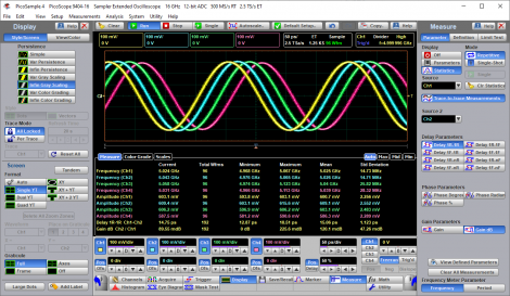
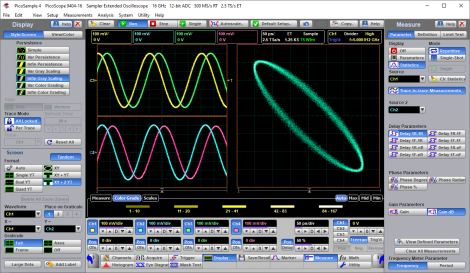
Categories and math operators Arithmetic: Add, Subtract, Multiply, Divide, Ceil, Floor, Fix, Round, Absolute, Invert, Common, Rescale.
Algebra: Exponentiation (e), Exponentiation (10), Exponentiation (a), Logarithm (e), Logarithm (10), Logarithm (a), Differentiate, Integrate, Square, Square Root, Cube, Power (a), Inverse, Square Root of the Sum.
Trigonometry: Sine, Cosine, Tangent, Cotangent, ArcSine, Arc Cosine, ArcTangent, Arc Cotangent, Hyperbolic Sine, Hyperbolic Cosine, Hyperbolic Tangent, Hyperbolic Cotangent.
FFT: Complex FFT, FFT Magnitude, FFT Phase, FFT Real part, FFT Imaginary part, Complex Inverse FFT, FFT Group Delay. Bit operator: AND, NAND, OR, NOR, XOR, XNOR, NOT.
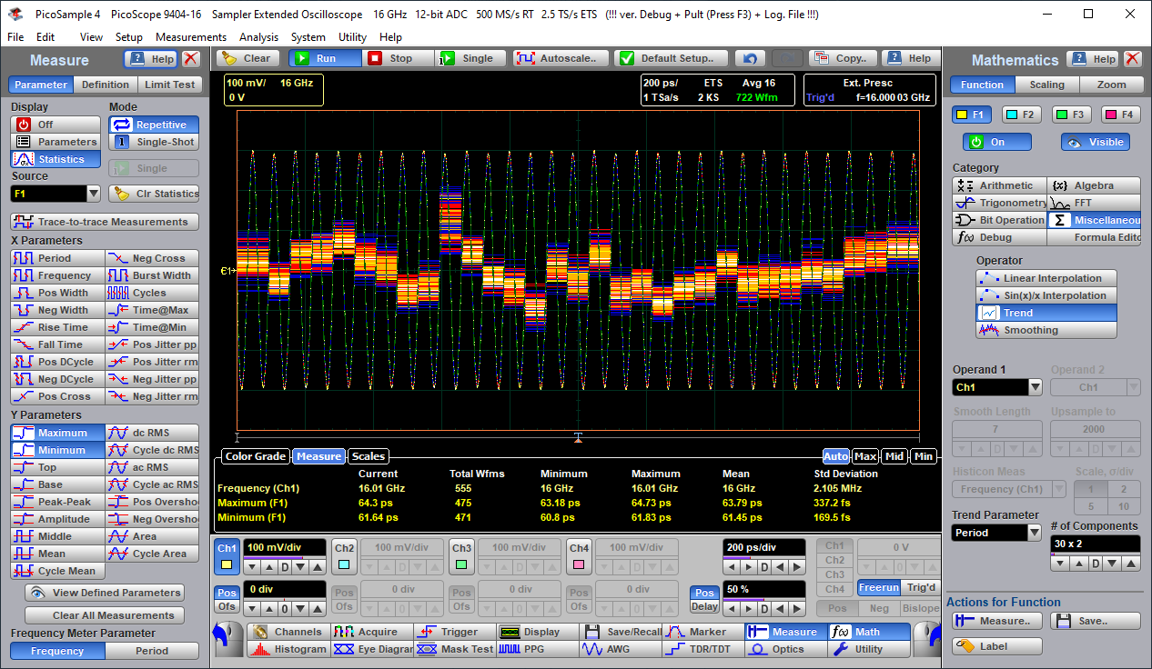
Miscellaneous: Autocorrelation, Correlation, Convolution, Track, Trend, Linear Interpolation, Sin(x)/x Interpolation, Smoothing.
Formula editor: Build math waveforms using the Formula Editor control window.
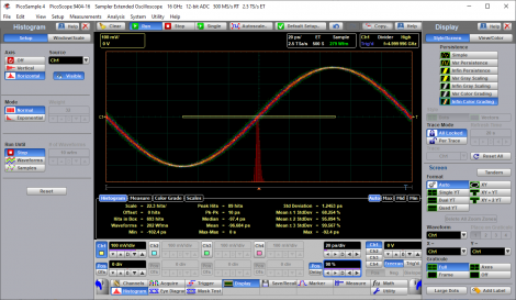
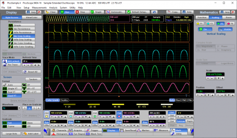
Operands Any channel, waveform memory, math function, spectrum, or constant can be selected as a source for one of two operands.
FFT FFT frequency span: Frequency Span = Sample Rate / 2 = Record Length / (2 × Time base Range) FFT frequency resolution: Frequency Resolution = Sample Rate / Record Length
FFT windows: The built-in filters (Rectangular, Hamming, Hann, Flattop, Blackman–Harris and Kaiser–Bessel) allow optimization of frequency resolution, transients, and amplitude accuracy.
FFT measurements: Marker measurements can be made on frequency, delta frequency, magnitude, and delta magnitude. Marker measurements can be made on frequency, delta frequency, magnitude, and delta magnitude.
Automated FFT Measurements include: FFT Magnitude, FFT Delta Magnitude, THD, FFT Frequency, and FFT Delta Frequency.
Histogram
Histogram axis Vertical, Horizontal or Off.
Both vertical and horizontal histograms, with periodically updated measurements, allow statistical distributions to be analyzed over any region of the signal.
Histogram measurement set Scale, Offset, Hits in Box, Waveforms, Peak Hits, Pk-Pk, Median, Mean, Standard Deviation, Mean ±1 Std Dev, Mean ±2 Std Dev, Mean ±3 Std Dev, Min, Max-Max, Max.
Histogram window The histogram window determines which part of the database is used to plot the histogram. You can set the size of the histogram window to be any size that you want within the horizontal and vertical scaling limits of the scope.
Eye diagram
Eye diagram The PicoScope 9400 can automatically characterize an NRZ and RZ eye pattern. Measurements are based upon statistical analysis of the waveform.
NRZ measurement set X: Area, Bit Rate, Bit Time, Crossing Time, Cycle Area, Duty Cycle Distortion (%, s), Eye Width (%, s), Fall Time, Frequency, Jitter (p-p, RMS), Period, Rise Time
Y: AC RMS, Crossing %, Crossing Level, Eye Amplitude, Eye Height, Eye Height dB, Max, Mean, Mid, Min, Negative Overshoot, Noise p-p (One, Zero), Noise RMS (One, Zero), One Level, Peak-Peak, Positive Overshoot, RMS, Signal-to-Noise Ratio, Signal- to-Noise Ratio dB, Zero Level.
RZ measurement set X: Area, Bit Rate, Bit Time, Cycle Area, Eye Width (%, s), Fall Time, Jitter P-p (Fall, Rise), Jitter RMS (Fall, Rise), Negative Crossing, Positive Crossing, Positive Duty Cycle, Pulse Symmetry, Pulse Width, Rise Time
Y: AC RMS, Contrast Ratio (dB, %, ratio), Eye Amplitude, Eye High, Eye High dB, Eye Opening Factor, Max, Mean, Mid, Min, Noise P-p (One, Zero), Noise RMS (One, Zero), One Level, Peak-Peak, RMS, Signal-to-Noise, Zero Level.
Mask test
Mask test Acquired signals are tested for fit outside areas defined by up to eight polygons. Any samples that fall within the polygon boundaries result in test failures. Masks can be loaded from disk, or created automatically or manually.
Mask creation Create the following masks: Standard predefined Mask, Automask, Mask saved on disk, Create new mask, Edit any mask.
Standard mask Standard predefined optical or standard electrical masks can be created.
SONET/SDH: OC1/STMO (51.84 Mb/s) to FEC 2666 (2.6666 Gb/s)
Fibre Channel: FC133 Electrical (132.8 Mb/s) to FC2125E Abs Gamma Tx.mask (2.125 Gb/s) Ethernet: 100BASE-BX10 (125 Mb/s) to 3.125 Gb/s 10GBase-CX4 Absolute TP2 (3.125 Gb/s) Infiniband: 2.5G InfiniBand Cable mask (2.5 Gb/s) to 2.5G InfiniBand Receiver mask (2.5 Gb/s) InfiniBand (2.5 Gb/s)
XAUI: 3.125 Gb/s XAUI Far End (3.125 Gb/s) to XAUI-E Near (3.125 Gb/s)
ITU G.703: DS1, 100 Ω twisted pair (1.544 Mb/s) to 155 Mb 1 Inv, 75 Ω coax (155.520 Mb/s) ANSI T1/102: DS1, 100 Ω twisted pair, (1.544 Mb/s) to STS3, 75 Ω coax, (155.520 Mb/s)
RapidIO: RapidIO Serial Level 1, 1.25G Rx (1.25 Gb/s) to RapidIO Serial Level 1, 3.125G Tx SR (3.125 Gb/s)
PCI Express: R1.0a 2.5G Add-in Card Transmitter Non-Transition bit mask (2.5 Gb/s) to R1.1 2.5G Transmitter Transition bit mask (2.5 Gb/s) Serial ATA: Ext Length, 1.5G 250 Cycle, Rx Mask (1.5 Gb/s) to Gen1m, 3.0G 5 Cycle, Tx Mask (3 Gb/s)
Mask margin Available for industry-standard mask testing
Automask creation Masks are created automatically for single-valued voltage signals. Automask specifies both delta X and delta Y tolerances. The failure actions are identical to those of limit testing.
Data collected during test Total number of waveforms examined, number of failed samples, number of hits within each polygon boundary
Calibrator output
Calibrator output mode DC, 1 kHz square, meander with frequency from 15.266 Hz to 500 kHz.
Output DC level Adjustable from –1 V to +1 V into 50 Ω. Coarse increment: 50 mV, fine increment: 1 mV.
* Output DC level accuracy ±1 mV ±0.5% of output DC level
Output impedance 50 Ω nominal
Rise/fall time 150 ns, typical
Output connectors SMA female
Trigger output
Timing Positive transition equivalent to acquisition trigger point. Negative transition after user holdoff.
Low level (–0.2 ±0.1) V. Measured into 50 Ω.
Amplitude (900 ±200) mV. Measured into 50 Ω.
Rise time 10% to 90%: ≤ 0.45 ns
20% to 80%: ≤ 0.3 ns
RMS jitter 2 ps or less
Output delay 4 ±1 ns
Output coupling DC coupled
Output connectors SMA female
9404-05 9404-16
Clock recovery trigger – recovered data output (optional)
Data rate 6.5 Mb/s to 5 Gb/s 6.5 Mb/s to 8 Gb/s
Eye amplitude 250 mV p-p, typical
Eye rise/fall time 20%–80%: 75 ps, typical. Measured at PicoScope 9404-05 20%–80%: 50 ps, typical. Measured at PicoScope 9404-16
RMS jitter 2 ps +1% of unit interval, typical 2 ps +1% of unit interval, typical
Output coupling AC-coupled AC-coupled
Output connections SMA female SMA female
9404-05 9404-16
Clock recovery trigger – recovered clock output (optional)
Output frequency Full rate clock output, 3.25 MHz to 2.5 GHz Full rate clock output, 3.25 MHz to 4 GHz
Output amplitude 250 mV p-p, typical 250 mV p-p, typical
Output coupling AC-coupled AC-coupled
Output connectors SMA female SMA female
9404-05 9404-16
Power requirement
Power supply voltage +12 V ±5%
Power supply current 2.6 A max. 3.3 A including accessories. 2.7 A maximum and 3.3 A inclusive of active accessory loadings
Protection Auto shutdown on excess or reverse voltage
AC-DC adaptor Universal adaptor supplied
PC connection
PC connection USB 2.0 (high speed). Also compatible with USB 3.0.
LAN.
Physical characteristics
Dimensions Width: 245 mm
Height: 60 mm
Depth: 232 mm
Net weight 1.4 kg
Environmental conditions
Temperature Operating, normal operation: +5 °C to +40 °C
Operating, for quoted accuracy: +15 °C to +25 °C
Storage: –20 °C to +50 °C
Humidity Operating: Up to 85 %RH (non-condensing) at +25 °C.
Storage: Up to 95 %RH (non-condensing).

* Specifications marked with (*) are checked in the Performance Verification chapter of the User’s Guide.
[1] These specifications are valid after a 30-minute warm-up period and ±2 °C from firmware calibration temperature.

Models

Discover out models range

9404-05 9404-16
16 GHz oscilloscope
5 GHz oscilloscope
Accessories included
Price €13 275 €22 575
Buy now Buy Buy
9404-05 9404-16