/
Products
/
Digital Storage Oscilloscopes
/
FemtoScope 1000/2000/3000

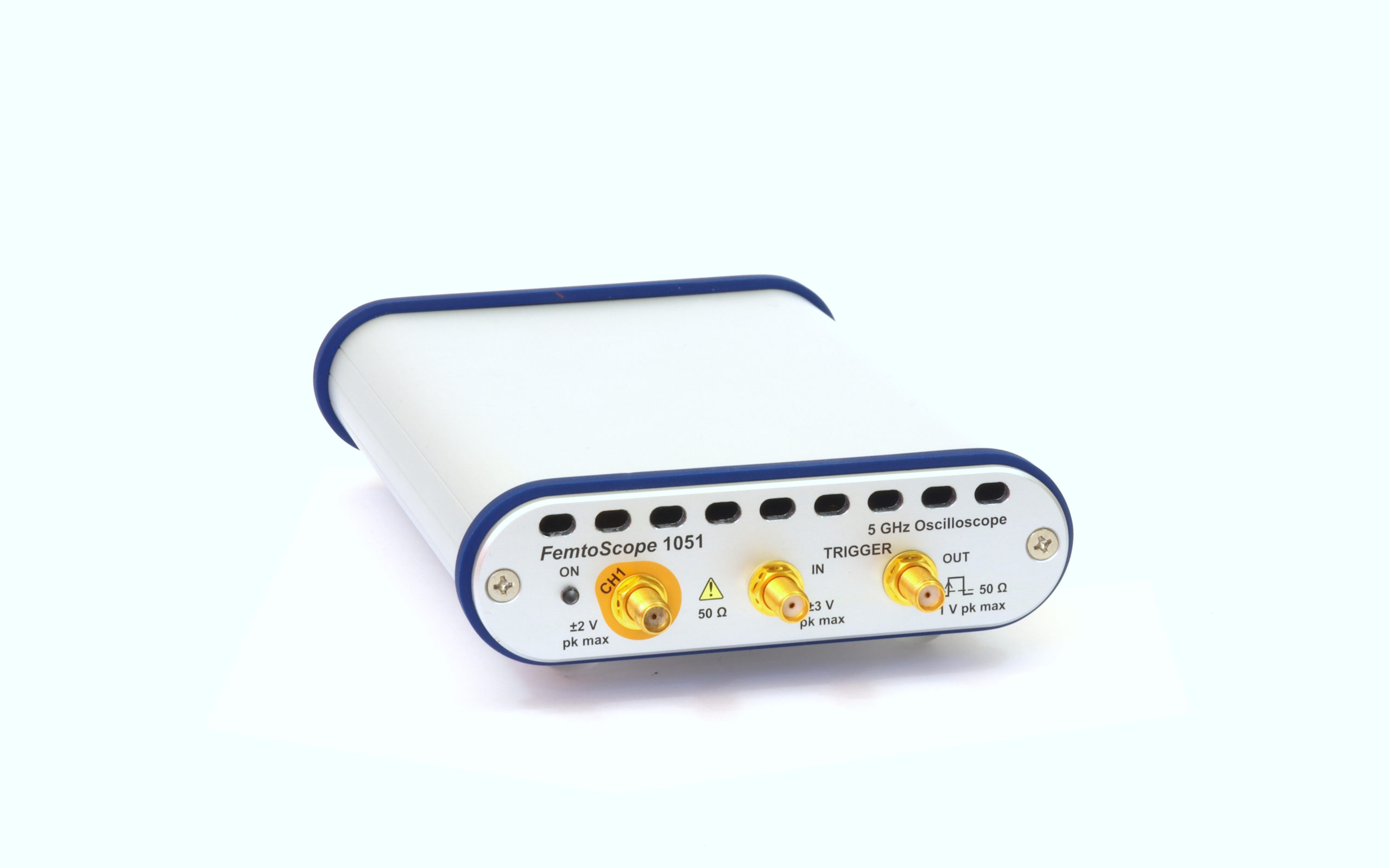
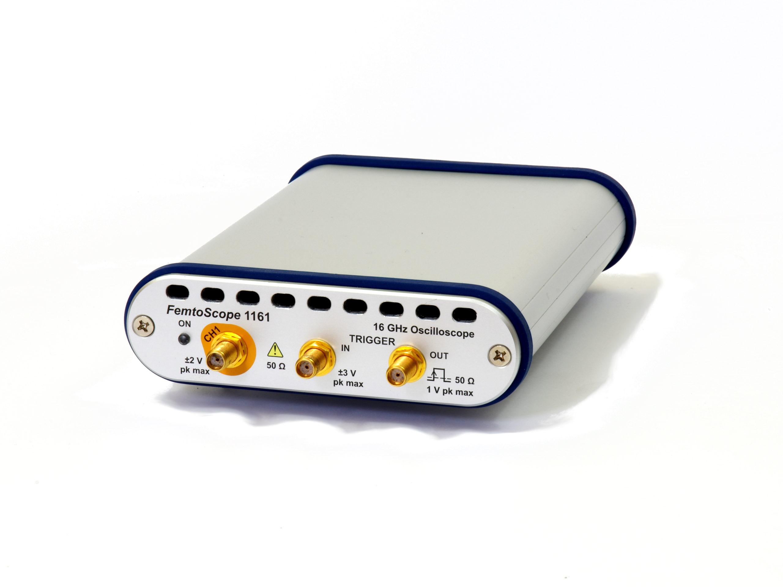
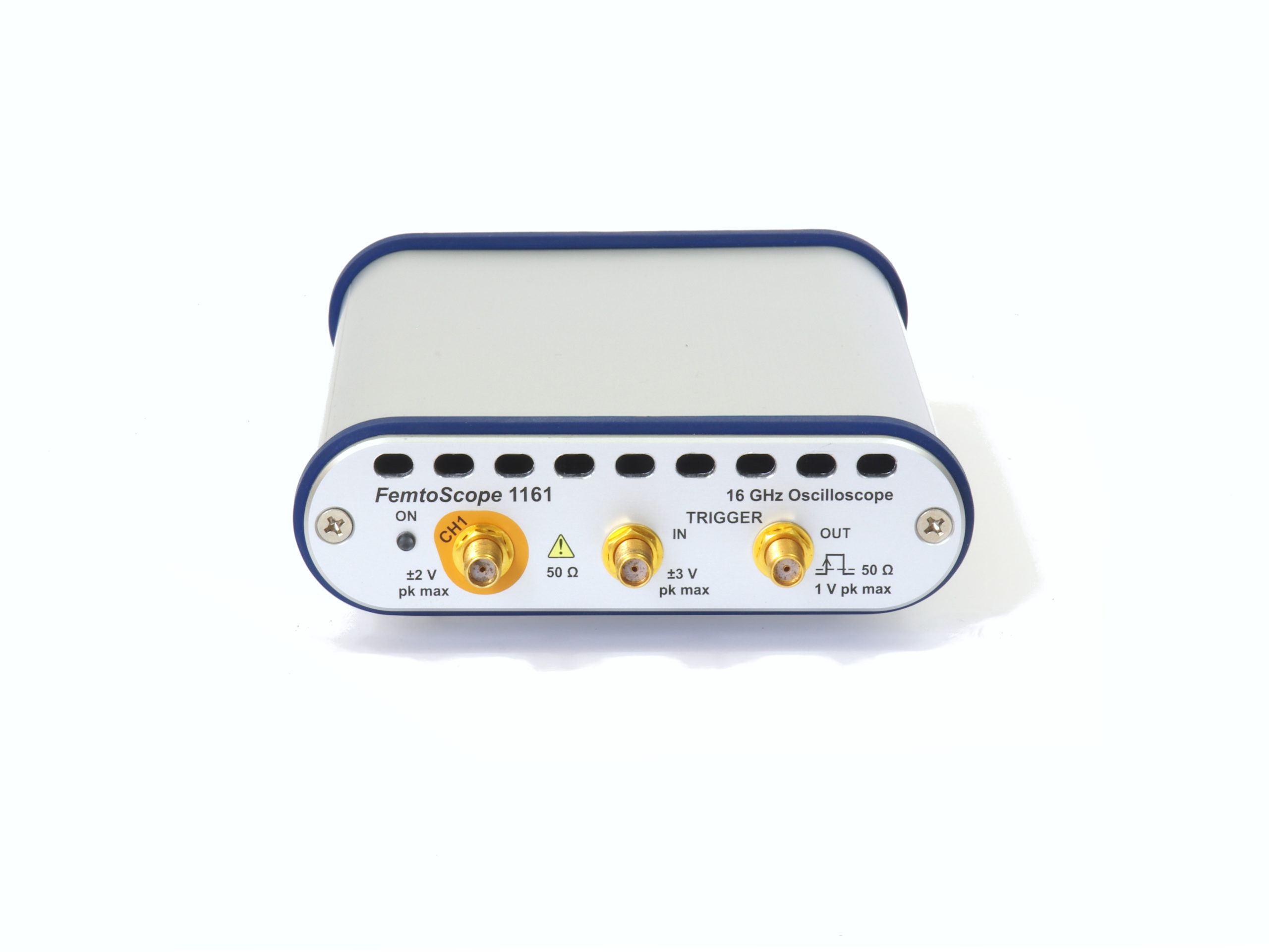
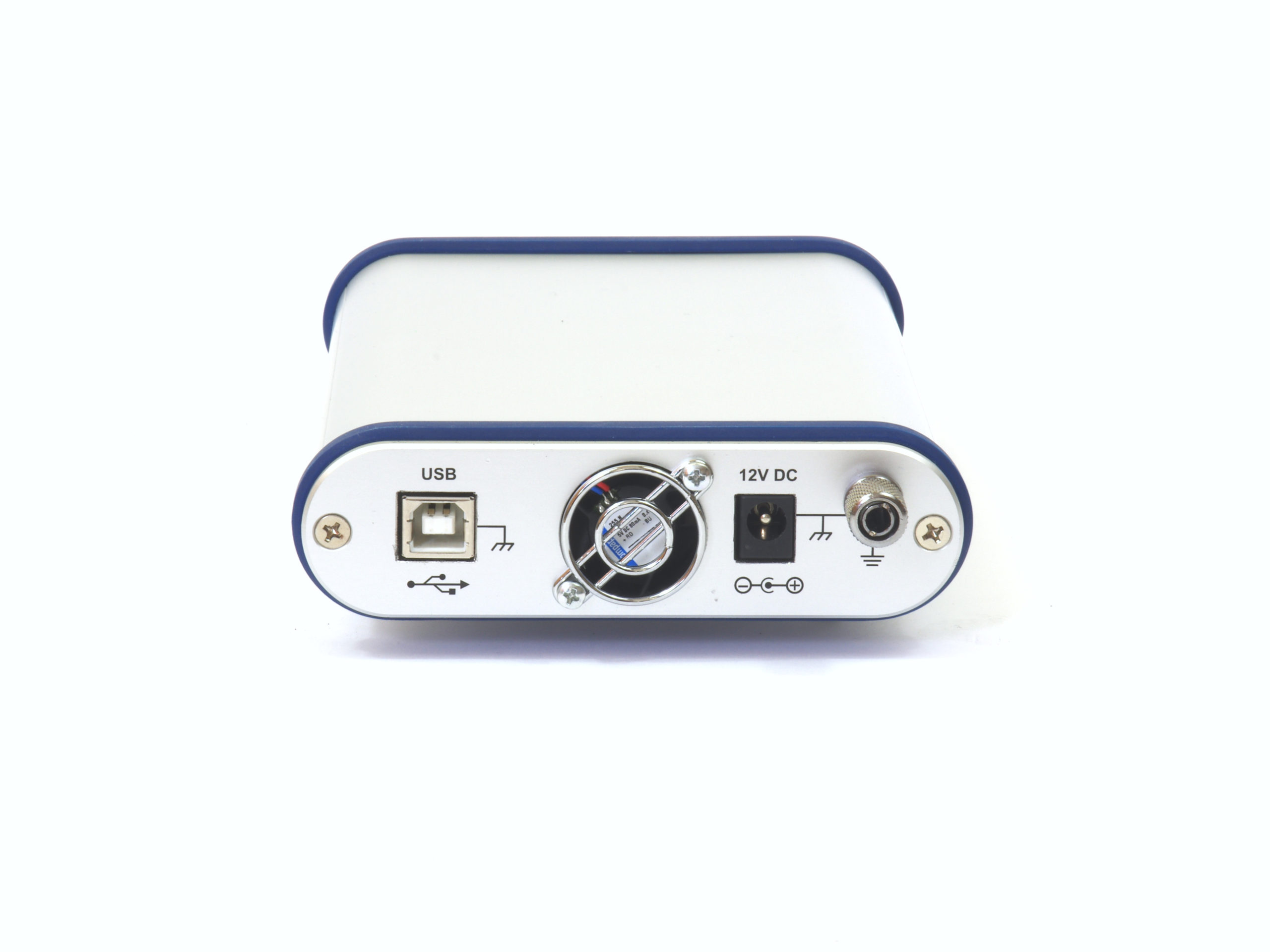
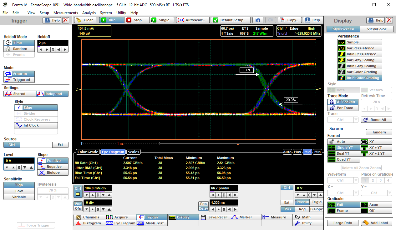
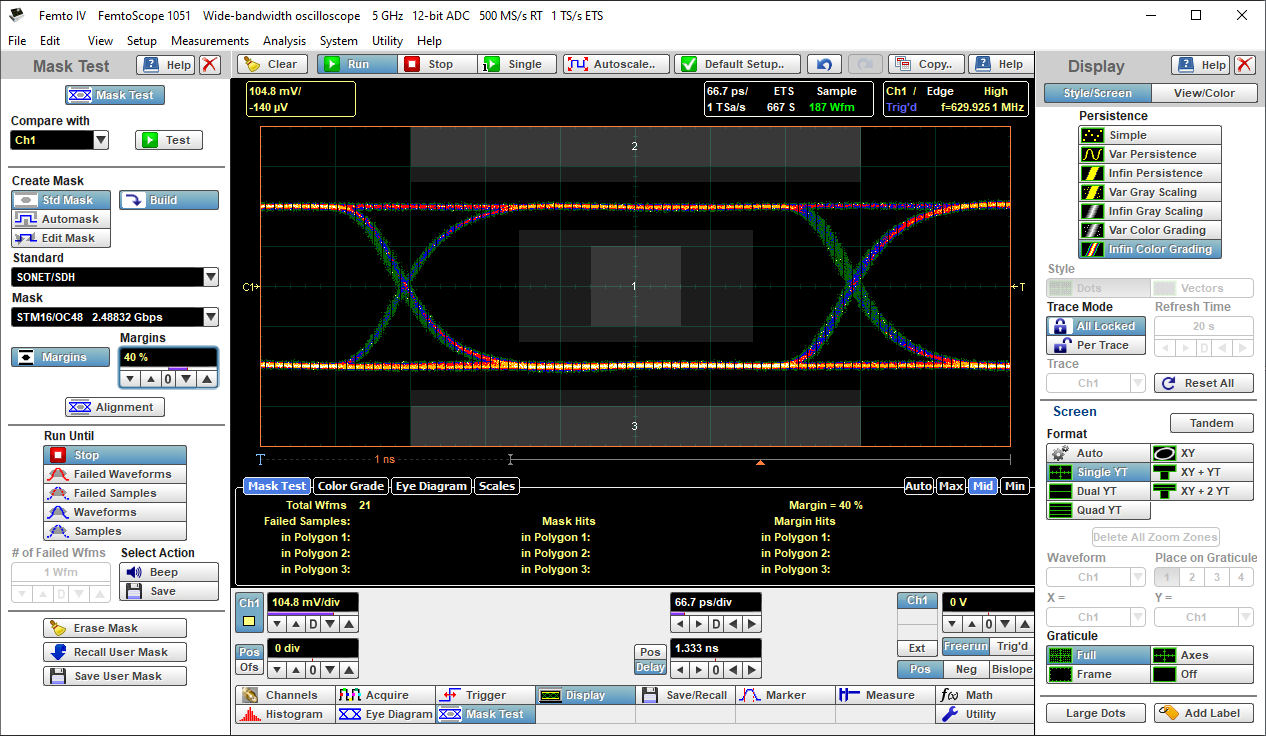
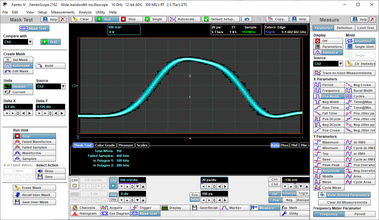
FemtoScope 1000/2000/3000

5 or 16 GHz bandwidth
4, 2 or 1 channels
500 MSa/s RT sampling rate
Up to 5 TSa/s ET sampling rate

The FemtoScope 1000, 2000 and 3000 series are portable and low cost digital storage oscilloscopes having bandwidth up to 5 or up to 16 GHz. These oscilloscopes are designed for engineers working both in research laboratories and in production workshops, and who, above all, need characteristics associated with flexible measurements of wide-bandwidth single-shot or repetitive signals.

Wide-Bandwidth Oscilloscopes for precise measurement and analysis

More recently, if you needed an oscilloscope with a bandwidth of more than 5 GHz, you had to accept the need for significant financial costs. The FemtoScope models set a new price/performance ratio standard for gigahertz frequency USB oscilloscopes.

These single-, dual- or four-channel instruments, having a bandwidth of 5 or 16 GHz and triggering over the entire frequency range, provide the acquisition, display, measurement and analysis of complex waveforms in the range from picoseconds to hundreds of seconds.

Being a direct alternative to traditional benchtop oscilloscopes, these instruments are portable, and maybe even miniature, and, what is extremely important, they have an incomparably lower cost. Economical prices make the FemtoScope Series preferred for teaching basic scientific and engineering measurements at lab stations in schools and universities. Features normally only found on much higher priced scopes equip the FemtoScope Series to be a powerful choice for R&D applications.

1, 2 or 4 channels configuration.
The industry’s widest 5 or 16 GHz USB oscilloscope bandwidths available to match your measurement application,
The industry’s lowest 1.5 ps rms typical intrinsic jitter for USB oscilloscope.
12-bit Analog-to-Digital Converter with 500 MSa/s real time sampling rate per channel.
The industry’s highest equivalent time sampling rate up to 5 TSa/s for USB oscilloscope.
10 ps/div fastest time base scale.
Up to 16 GHz trigger bandwidth enables capture and analysis wide-bandwidth complex signals.
Up to 11.3 Gb/s clock recovery trigger data rate.
Powerful SW and flexible, simple and intuitive user interface with built-in OnLine Help and demo training signals.
Color graded display, automatic measurements, eye diagrams, mask test, histograms, waveform mathematics, 7-digit built-in frequency counter, spectrum analysis with FFT, autoscale, store waveforms and setups.
Power consumption less than 15 or 22 W.
Weight less than 370 or 790 grams.
Footprint less than 1.9 or 3.4 sq.dm.
Economical price.

The FemtoScope USB oscilloscopes utilize modern hardware to perform many of the functions that traditional digitizers do with software on the CPU. Built as a single-board oscilloscope, they are controlled from a computer via USB interface. Acquisition Board includes ultra-wideband track-and-hold amplifiers, 12-bit ADCs with 500 MSa/s sampling rate, high-speed trigger circuity and timing interpolator with sub-picosecond resolution. A state-of-the-art microprocessor, FPGA and precision clock oscillator provide structure flexibility, fast acquisition speed and effective interaction with PC.

Bandwidth and transient response

The FemtoScope 1000/2000/3000 series USB oscilloscopes have one, two or four input channels up to 5 or 16 GHz with market-leading ADC, timing and display resolutions for accurately measuring and visualizing high-speed analog and data signals. They are ideal for capturing pulse and step transitions down to 70 or 22 ps, impulses down to 140 or 45 ps and clocks and data eyes to 5 or 11.3 Gb/s. Most high-bandwidth applications involve repetitive signals or clock-related data streams that can be readily analyzed with these oscilloscopes by equivalent-time sampling.
Figure on the right shows frequency response of twelve channels (six oscilloscope) measured on the FemtoScope 2162.

The other figure on the right shows transient response of the FemtoScope 2162 tested with Keysight N2806A Calibration Generator. Total measured fall time is 23.71 ps, rms jitter is 1.256 ps, and negative overshot is 5.495%

The heart of each of the channel is a wide-bandwidth track-and-hold amplifier, which stores the analog voltage at the channel input at a time determined by the arrival of a 500-MHz sampling pulse. The inputs include wide-bandwidth symmetrical resistive voltage divider. One half of the signal goes to the THA, the other to the trigger comparator. The input impedance of the channel is (50 ± 1.5) Ohms. With a maximum permissible input voltage of ±2 V, the dynamic range of the input signals is ±1 V.

User-selectable hardware bandwidth-limiting reduces vertical noise. More bandwidth enhances quality of your measurements except when you want to limit noise level coming from additional bandwidth. However wide bandwidth may not be the best solution when you are making low-noise measurements as the additional bandwidth captures additional high-frequency noise along with high-frequency signal content.
All four models of oscilloscopes provide two bandwidth modes full bandwidth or low bandwidth 450 MHz.. Their transient response characteristics are shown in figures on the right.

Vertical channels and probes

Providing up to 12 bits of vertical resolution the FemtoScope allow to control vertical sensitivity between 10 mV/div and 250 mV/div. Full scale is defined as 8 vertical divisions, and further zooming may increase sensitivity in 100 times. With ±1.5% DC gain accuracy and ±1 V DC offset the scopes provide wide input dynamic range between -1 V and +1 V.

Figure on the right shows 1.9 V amplitude pulse symmetrical to zero. With rise time faster than 10 ns it has very small ringing within ±1 %.
With 50 Ω channel input impedance oscilloscopes used standard SMA female connector providing ±2 V (DC + peak AC) maximum input voltage.
You can use wide range of high-bandwidth low-impedance probes. The PicoConnect 900 family of high performance, ultra-low capacitance passive probes tailored to low invasive probing of high speed data lines out to 18 Gb/s (9 GHz). They are ideal companions for the FemtoScope Series, allowing cost-effective fingertip browsing of fast signals.

Two series are available: RF, microwave and pulse probes for broadband signals up to 5 GHz (10 Gb/s), and Gigabit probes for data streams such as USB 2, HDMI 1, Ethernet, PCIe and SATA up to 9 GHz (18 Gb/s).

Acquisition and time base

The FemtoScope oscilloscopes used real-time, equivalent-time and roll sampling modes.
Real-time sampling mode is designed with a high enough sampling rate to capture a transient, non-repetitive signal with the instrument’s specified analog bandwidth up to 250 MHz. According to Nyquist’s sampling theorem, for accurate capture and display of the signal the scope’s sampling rate must be at least twice the signal bandwidth. Typical high-bandwidth real-time oscilloscopes exceed this sampling rate by perhaps a factor of two, achieving up to four samples per cycle, or three samples in a minimum-width impulse.
Several acquisition modes let you choose how the oscilloscope will create points in the waveform record. Average calculates the average values for each record point over many waveform records. It is available in in real- and equivalent-time modes. Min-Max, Min and Max Envelope use the highest and lowest samples across several waveform records. These are also available in real- and equivalent-time modes. Peak Detect mode alternates between saving the highest sample in one acquisition interval and the lowest sample in the next acquisition interval. It is available in real-time only. High Resolution mode averages all samples taken during an acquisition interval to create a record point. This average results in a higher-resolution, lower-bandwidth waveform that works with real-time mode.
Time scale accuracy is critical, especially when you need deep-memory applications. In real-time acquisition the FemtoScope used internal precise 500 MHz clock that allows 10 ns/div faster time base scale.

Stability of real-time clock can be estimated as a „long-time” jitter. Figure on the right demonstrates 716 ps rms jitter measured at 100 ms horizontal delay. This is equivalent to 7.16 ppb real-time rms jitter.

For signals close to or above Nyquist limit, the FemtoScopes can be switched into equivalent-time sampling mode. In this mode the scope acquires as many samples as it can for each of many trigger events, each trigger contributing more and more samples and detail in a reconstructed waveform. Critical to alignment of these samples is a separate and precise measurement of time between each trigger and the next occurring sample clock. After a large number of trigger events the scope has enough samples to display the waveform with the desired time resolution. This is called the effective sampling resolution, which is many times higher than is possible in real-time mode. As an example 16-GHz FemtoScope models have 0.2 ps timing resolution that is equivalent to 5 TSa/s equivalent-time sampling rate. While 5-GHz models have 1 ps timing resolution that is equivalent to 1 TSa/s.
As this technique relies on a random relationship between trigger events and the sampling clock, it is more correctly called random equivalent-time sampling (or sometimes random interleaved sampling, RIS). It can be used for repetitive signals or for data pattern when you want to build an eye diagrams.
Equivalent-time sampling mode is the most actual for signal integrity measurements when you need very accurate results for such parameters as rise time or jitter. Precise picosecond time base and low intrinsic trigger jitter are necessary for ensuring high-speed test system reliability. With more lower the value, the better you’ll be able to characterize your device. Figure on the right shows how the FemtoScope 2162 measures accuracy of 10-GHz sinewave (period=100 ps) in equivalent time sampling with timing resolution of 0.2 ps.

Zoom

Due to the long memory, the zoom allows you to view and compare up to four vertically and horizontally enlarged waveform sections simultaneously. At the same time, it is possible to shift any of zoomed zones both vertically and horizontally. The maximum vertical zoom is 100, and maximum horizontal zoom is 2048.

Figure on the right demonstrates 50 Mb/s data pattern acquired at 500 MSa/s sampling rate, 50 us/div time base scale and 250 KB record length (top). With 2K horizontal zoom you have possibility to measure the details of the waveform at 25 ns/div time base (bottom).

Trigger

All the models of the oscilloscopes provide full-function internal or external direct trigger up to 3 GHz. Input high-speed comparators allow you to adjust the trigger level and hysteresis, providing trigger sensitivity better than 50 mV. It is possible to select any of the trigger slope, as well as use the bi-slope trigger, which allows you to acquire the so-called pseudo-eye diagrams.
To expand the trigger frequency range up to 6 GHz, the FemtoScope models provides a frequency divider mode. This mode is especially relevant for measurements on such popular clock ranges as 3.25 GHz and 5 GHz.

Finally the FemtoScope 2162 and 3164 provide external prescaled trigger within full 16-GHz bandwidth. This trigger is realized by using high-frequency divider. The divider has fixed division factor of 8, as well as a small additive phase noise, which helps to achieve a low trigger jitter level. Figure on the right shows how the FemtoScope 2162 provides external prescaled trigger from 16 GHz sinewave with 1.37 ps rms jitter

Frequency counter

A dedicated frequency counter shows signal frequency (or period) at all times, regardless of measurement and time base settings, with a 7 digits resolution. For FemtoScope 2162 and 3164 maximum frequency is 16 GHz, for other four models it is 6 GHz.

Connectivity

Built-in USB device ports make PC connectivity easy for all models of the oscilloscopes. To provide a confident connectivity you need USB cable and external AC/DC power adapter (no power is used from the USB connection). Both parts are included in the oscilloscope kit.

The FemtoScope 3000 used both USB and LAN ports.

Portability

Weighing less than 370 g with a 1.9 sq.dm small footprint, the FemtoScope 1000 Series USB oscilloscopes can go anywhere with ease. You can just put it in the pocket of your jacket or in a small briefcase
New FemtoScope 2000 Series USB oscilloscopes deliver the performance and features you expect in a big scope. 16 GHz bandwidth on two channels, less than 2 ps rms jitter, 8 Gb/s clock recovery trigger are now available with portable enclosure having less than 790 g weight and 3.4 sq.dm small footprint.

Standard accessories

Your FemtoScope Series oscilloscope kit contains the following items:
• FemtoScope USB Wide-Bandwidth Oscilloscope.
Specified from FS1051, FS1161, FS2051, FS2162, FS3054 or FS3164.
• Femto IV software (supplied on a USB stick and also available as a free download from www.eltesta.com).
• Quick start guide (supplied on a USB stick and also available as a free download from www.eltesta.com)..
• 12 VDC power supply with specified localized IEC mains lead.
• 80 cm precision cable, 2 pcs.
• USB cable, 1.8 m.
• SMA / PC3.5 / 2.92 wrench.

Automatic measurements

The FemtoScope oscilloscopes provide a wide range of automatic measurements. More than 50 types of typical automatic oscilloscope measurements give you quick access to powerful functions. They are separated into four categories: amplitude, time, inter-channel and spectral measurements. Each of the measurement can be performed on live signals, saved waveforms or math functions.

Up to 10 measurements continuously updated with statistics. With statistical measurements, the oscilloscope measures the minimum, maximum, average and current values, as well as the standard deviation. Amplitude measurements include 17 parameters such as maximum, minimum, top, base, peak-peak, amplitude, middle, mean, cycle mean, rms, etc. 18 timing measurements include period, frequency, positive or negative pulse width, rise or fall time, duty cycle, etc. Inter-channel measurements are those performed on two signals. These include delay, phase, and gain. Spectral measurements are performed with FFT and include FFT magnitude and delta magnitude, total harmonic distortion, FFT frequency and delta frequency.

Histogram

Histograms are a statistical representation of a signal or its measurement results. The FemtoScope oscilloscopes use two types of histograms – vertical and horizontal. You can turn on the histogram to live signals, saved wave forms or math functions. Color grade display usually used with histogram on a waveform to add statistical view.
A vertical histogram is a probabilistic distribution of data collected about a signal along a vertical axis within a given histogram window. The information collected by such a histogram is used in the statistical analysis of the signal source. A vertical histogram is the most acceptable way to measure the noise characteristics of the wave forms. Noise is measured by sizing the histogram window to a narrow portion of time and observing a vertical histogram that measures the noise on an edge.

The parameters of both the vertical and horizontal histograms include the display scale in hits per division or dB per division, the offset in hits or dB (the number of hits or dB at the bottom of the display, as opposed to the center of the display), the total number of samples included in the histogram box, the number of wave forms that have contributed to the histogram, the number of hits in the histogram’s greatest peak, the width, median and mean of histogram, the standard deviation (σ) value of the histogram, also the percentage of points that are within ± 1σ, ± 2σ and ± 3σ of the mean value, etc.
The most common uses for horizontal histogram is measuring and characterizing timing jitter on displayed wave forms. Jitter is measured by sizing the histogram window to a narrow portion of voltage and observing a horizontal histogram that measures the jitter on an edge.

Eye Diagram

An eye diagram is an effective graphical method for evaluating the quality of a digital pattern. The results of its measurements are integral characteristics that describe the quality of the data channel and its ability to reproduce waveforms in undistorted form. Eye diagram helps to visualize signal integrity.
The relationship between the required oscilloscope bandwidth and the maximum data rate is known. To acquire the third harmonic of the stream, this ratio is 1.8, and for the fifth harmonic it is already 3.

Following these relationships 16-GHz Femtoscope will acquire the third harmonic of the 8.8 Gb/s data pattern and the fifth harmonic of the 5.3 Gb/s data pattern. At the same time 5-GHz Femtoscope will acquire the third harmonic of the 2.5 Gb/s data pattern and the fifth harmonic of the 1.7 Gb/s data pattern.
In general, eye diagrams are multilevel waveforms. The FemtoScopes measures two-level eye diagrams, such as NRZ (“No return to zero”) or RZ (“Return to zero”).

A high-quality eye diagram on the FemtoScope screen can be obtained in two ways. The first method is available when measuring data pattern is fed to the channel input, and it is also selected as the synchronization source. “Clock recovery” should be selected as the trigger style. With this method, the data rate range reaches 11.3 Gb/s for the FS2162 or FS3164, and 5 Gb/s for FS2052 or FS3054 models.
The second way is that the measuring data pattern is fed to the input of the channel, and the clock signal used as a trigger source is supplied to another channel or to the input of any of external trigger input. In principle, the second method does not need to use clock recovery style.

You can reach data rate up to 16 Gb/s for the FS2162 or FS3164, and 6 Gb/s for other four models. In order to make the correct measurements, the eye diagram is automatically autoscaled so that its vertical size is four large divisions, its horizontal size is six large divisions.

Eye-diagram measurements include such parameters as eye height, eye width, jitter rms, crossing percentage, Q factor, and duty-cycle distortion. Totally the FemtoScope can measure 27 vertical and 15 horizontal parameters of NRZ eye diagram, ten of them can be measured simultaneously.
The FemtoScope also allows you to measure 26 vertical and 17 horizontal parameters of the RZ eye diagram.

Mask Test

This test is used when it is necessary to control the shape of the measured waveform. Such waveforms can be quite complex as, and example, eye diagrams, and the number of possible waveform anomalies can be significant, which makes it difficult to perform standard measurements.
Mask test is widely used in production, in the control of quality, as well as in its testing for compliance with the requirements of standards. It is useful when you need to validate the stability of your electronic components and systems.
The test works on a good / bad basis.
Masks are geometric templates that show acceptable areas of the screen into which testing waveform should not fall. The FemtoScope uses three types of masks – standard, automatic and arbitrary.
The shape of standard masks depends on the type of standard and its data rate. The oscilloscopes will allow to analyze standard masks of the following international standards – SONET / SDH, Ethernet, RapidIO, G.984.2, Fiber Channel, ITU G.703, PCI Express, ANSI T1.102, InfiniBand, Serial ATA and XAUI. The shape of standard masks is usually a quad or hexagon. There are options for editing standard masks.
Depending on bandwidth specifications the FemtoScope provide up to 161 types of standard masks.
The principle of mask test is to determine if the waveform hits the mask, which violates the boundaries of the mask. Such a hit detects the exceeding the specified limits. This is fixed by changing the color of the waveform to red, which indicates an error in its shape.
Statistical test results include information about errors registered within standard templates, registered within additional margins, as well as full error information.

Other commonly used is an automask. An automatic mask is constructed according to the shape of tested waveform by adding to it certain preset tolerances vertically and horizontally.
Figure on the right shows an automatic mask constructed for a short 80-ps pulse. The mask consists of two patterns that seamlessly repeat the waveform on both sides of it. Figure also shows an automask test under the influence of noise. Acquired points on a pulse that go beyond tolerances are marked in red. In this example, horizontal tolerance limit is ±5 ps.
The last is arbitrary type of mask. It can be created directly by the user. Moreover, the number of templates can be up to eight, and their shape can be freely edited and saved.

Mathematics

Based on the data on acquired waveform, the FemtoScope allows the simultaneous calculation of up to four mathematical functions. Any mathematical function can be selected as an operator for one or two operands (sources). For example, inversion is a one-operand function, while addition is a two-operand function. Live waveforms, stored waveforms, or other mathematical functions can be selected as an operand.
The oscilloscopes used several categories of mathematical functions. These are arithmetic (12 functions), algebraic (14 functions), trigonometric (12 functions), spectral (6 functions), logical (7 functions), etc. It is also possible to use the formula editor.

Arithmetic functions include such functions as addition, subtraction, multiplication, division, absolute value, inversion, half-sum, scaling, etc. Algebraic functions include functions such as the exponent on the base e, 10 or on an arbitrary base, the logarithm, differentiation, integration, square, cube, square root, etc. Trigonometric functions include functions such as sine, cosine, tangent, cotangent, arcsine, arccosine, arctangent, arc tangent, hyperbolic tangent and hyperbolic cotangent.
FFT includes FFT magnitude and phase, the real and imaginary parts, also the inverse FFT. To compensate for the inherent limitations of the FFT, the operator must use the FFT windows. The type of window determines the bandwidth and slope of the corresponding mathematical filter. The oscilloscope supports six types of FFT windows. A rectangular FFT window does not change the signal data acquired in the time domain. Other five FFT windows have different filter characteristics in the time domain. They are Hamming window, Hanning window, flat window, Blackman-Harris window and Kaiser-Bessel window.
Logical functions include such functions as AND, AND-NOT, OR, OR-NOT, exclusive OR, exclusive OR-NOT, and also NOT.

In real time, when relation between sampling rate and the input frequency may significantly decrease, aliasing distortions occur. To avoid such distortions the oscilloscopes provide linear or Sin (x) / x interpolation functions. The Sin (x) / x interpolation function effectively restores the shape of the input signal.

The oscilloscopes used trend as a mathematical function that shows the nature of the variation in the signal parameter over time. The vertical axis shows the value of the selected parameter, and the horizontal axis shows the period of the signal for which this parameter was calculated.

Figure on the right is the example how the oscilloscope measures the period of the harmonic signal used to calibrate the sweep (purple). The trend function of the measured period (blue) is the mathematical function of this signal. Amplitude measurements of the trend function show the evolution of the change in the period value, i.e. show the magnitude of the non-linearity of the sweep at various horizontal points of the scale.

Please give us your feedback about FemtoScope 1000/2000/3000

Your opinion is very important to us. We appreciate your feedback and will use it to evaluate changes and make improvements in our products:

FemtoScope 1000/2000/3000 Downloads

Here you can download the latest FemtoScope 1000/2000/3000 Data Sheets, Manuals, Guides and other relevant documents:

Resources	Language	Version	Size	Updated
Data Sheets
FemtoScope 1000, 2000, 3000 Datasheet	English	2	5.37 Mb	2020
FemtoScope 1000, 2000, 3000 Specifications	English	2	399.55 Kb	2020
Software
Femto_IV_Setup	English	4.5.131	-	2020
Femto IV Setup 4.5.131	English	4.5.131	-	2021
Femto IV Setup 4.10.87	English	4.10.87	-	2023

Specifications and Characteristics

* Specifications marked with ( * ) are checked in the Performance Verification.

Vertical	FS1051	FS2052	FS3054	FS1161	FS2162	FS3164
Input channels	1	2	4	1	2	4
	All channels are identical and digitized simultaneously.
Analog bandwidth, –3 dB flatness	These specifications are valid after a 30-minute warm-up period and ±2 °C from firmware calibration temperature.
Full bandwidth *	DC to 5 GHz			DC to 16 GHz
Middle bandwidth, typical	N/A		DC to 500 MHz	N/A		DC to 500 MHz
Narrow bandwidth, typical	DC to 500 MHz		DC to 100 MHz	DC to 500 MHz		DC to 100 MHz
Passband flatness (full BW)	±1 dB to 3 GHz			±1 dB to 5 GHz
Calculated rise time (Tr), typical	Calculated from the bandwidth: 10% to 90%: calculated from Tr = 0.35/BW. 20% to 80%: calculated from Tr = 0.25/BW.
Full bandwidth	10% to 90%: ≤ 70 ps, 20% to 80%: ≤ 50 ps.			10% to 90%: ≤ 21.9 ps, 20% to 80%: ≤ 15.6 ps.
Middle bandwidth	N/A		10% to 90%: ≤700 ps 20% to 80%: ≤500 ps	N/A		10% to 90%: ≤700 ps 20% to 80%: ≤500 ps
Narrow bandwidth	10% to 90%: ≤ 700 ps 20% to 80%: ≤ 500 ps		10% to 90%: ≤3.5 ns 20% to 80%: ≤2.5 ns	10% to 90%: ≤ 700 ps 20% to 80%: ≤ 500 ps		10% to 90%: ≤3.5 ns 20% to 80%: ≤2.5 ns
Step response, typical
Full bandwidth				N/A
Overshoot	< 8%
Ringing	±6% to 3 ns, ±4% from 3 ns to 10 ns, ±3% from 10 ns to 100 ns, ±2% from 100 ns to 400 ns, ±1% after 400 ns.
Middle bandwidth	N/A			N/A
Overshoot			< 6%			< 6%
Ringing			±4% to 10 ns, ±3% from 10 ns to 100 ns, ±2% from 100 ns to 400 ns, ±1% after 400 ns.			±4% to 10 ns, ±3% from 10 ns to 100 ns, ±2% from 100 ns to 400 ns, ±1% after 400 ns.
Narrow bandwidth
Overshoot	< 6%		< 5%	< 6%		< 5%
Ringing	±4% to 10 ns, ±3% from 10 ns to 100 ns, ±2% from 100 ns to 400 ns, ±1% after 400 ns.		±5% to 20 ns, ±3% from 20 ns to 100 ns, ±2% from 100 ns to 400 ns, ±1% after 400 ns.	±4% to 10 ns, ±3% from 10 ns to 100 ns, ±2% from 100 ns to 400 ns, ±1% after 400 ns.		±5% to 20 ns, ±3% from 20 ns to 100 ns, ±2% from 100 ns to 400 ns, ±1% after 400 ns.
RMS noise
Full bandwidth *	1.8 mV, maximum. 1.6 mV, typical.			2.4 mV, maximum. 2.2 mV, typical.
Middle bandwidth	N/A		0.8 mV, maximum. 0.65 mV, typical.	N/A		0.8 mV, maximum. 0.65 mV, typical.
Narrow bandwidth	0.8 mV, maximum. 0.65 mV, typical.		0.6 mV, maximum. 0.45 mV, typical.	0.8 mV, maximum. 0.65 mV, typical.		0.8 mV, maximum. 0.65 mV, typical.
Scale factors (sensitivity)	10 mV/div to 250 mV/div. Full scale is 8 vertical divisions. Adjustable in a 10-12.5-15-20-25-30-40-50-60-80-100-125-150-200-250 mV/div sequence. Also adjustable in 1% fine increments or better. With manual or calculator data entry the increment is 0.1 mV/div.
DC gain accuracy *	±1.5% of full scale, maximum. ±1% of full scale, typical.		±1% of full scale, maximum. ±0.5% of full scale, typical.	±1.5% of full scale, maximum. ±1% of full scale, typical.		±1% of full scale, maximum. ±0.5% of full scale, typical.
Position range	±4 divisions from center screen
DC offset range	Adjustable from –1 V to +1 V in 10 mV increments (coarse). Also adjustable in fine increments of 2 mV. With manual or calculator data entry the increment is 0.01 mV for offset between –99.9 and 99.9 mV, and 0.1 mV for offset between –999.9 and 999.9 mV. Referenced to the center of display graticule.
DC offset accuracy *	±1.5 mV ± 1.5% of offset setting, maximum. ±1 mV ± 1% of offset setting, typical.		±1 mV ± 1% of offset setting, maximum. ±0.5 mV ± 0.5% of offset setting, typical.	±1.5 mV ± 1.5% of offset setting, maximum. ±1 mV ± 1% of offset setting, typical.		±1 mV ± 1% of offset setting, maximum. ±0.5 mV ± 0.5% of offset setting, typical.
Operating input voltage	±1 V
Vertical Zoom and Position	For all input channels, waveform memories, or functions.
Vertical factor	0.01 to 100.
Vertical position	±800 division maximum of zoomed waveform.
Channel-to-channel crosstalk (channel isolation)	≥50 dB (316:1) for input frequency DC to 1 GHz. ≥40 dB (100:1) for input frequency >1 GHz to 3 GHz. ≥36 dB (63:1) for input frequency >3 GHz to ≤5 GHz			≥50 dB (316:1) for input frequency DC to 1 GHz. ≥40 dB (100:1) for input frequency >1 GHz to 3 GHz. ≥36 dB (63:1) for input frequency >3 GHz to ≤16 GHz.
Delay between channels	N/A	≤ 10 ps typical at full bandwidth, equivalent time.		N/A	≤ 10 ps typical at full bandwidth, equivalent time.
ADC resolution	12 bits
Hardware vertical resolution	0.5 mV / LSB without averaging.
Input impedance *	50 Ω ± 1.5 Ω maximum. 50 Ω ± 1 Ω typical
Input match	Reflections for 70 ps rise time: 10% or less.			Reflections for 50 ps rise time: 10% or less.
Input coupling>	DC
Maximum safe input voltage	±2 V (DC + peak AC)
Input connector	SMA female
Attenuation	Attenuation factors may be entered to scale the oscilloscope for external attenuators connected to the channel inputs.
Range	0.0001:1 to 1 000 000:1
Units	Ratio or dB
Scale	Volt, Watt, Ampere, or Unknown.

Horizontal	FS1051	FS2052	FS3054	FS1161	FS2162	FS3164
Time base	Internal time base common to all input channels.
Time base range	Full horizontal scale is 10 divisions.
Real time sampling	10 ns/div to 1000 s/div.
Random equivalent time sampling	50 ps/div to 5 μs/div.			10 ps/div to 5 μs/div.
Roll	100 ms/div to 1000 s/div.
Segmented	Total number of segments: 2 to 1024. Dead time between segments: 3 µs.
Horizontal zoom and position	For all input channels, waveform memories, or functions
Horizontal factor	From 1 to 2000.
Horizontal position	From 0% to 100% non-zoomed waveform.
Time base clock accuracy	@ 25 ºC ± 3 ºC
Frequency	500 MHz
Initial set tolerance	± 0.5 ppm	± 5 ppm		± 0.5 ppm	± 5 ppm
Overall frequency stability * (over operating temperature range)	± 2 ppm		± 15 ppm	± 2 ppm		± 15 ppm
Aging	± 3 ppm		± 7 ppm	± 3 ppm		± 7 ppm
Time base resolution	1.0 ps			0.2 ps
	At random equivalent time sampling
Delta time measurement accuracy *	FemtoScope 1000: ± (2 ppm * reading + 0.1% * screen width + 5 ps). FemtoScope 2000: ± (15 ppm * reading + 0.1% * screen width + 5 ps). FemtoScope 3000: ± (15 ppm * reading + 0.1% * screen width + 2 ps).
Pre-trigger delay	Record length / current sampling rate maximum at zero variable delay time
Post-trigger delay	0 to 4.28 s. Coarse increment is one horizontal scale division, fine increment is 0.1 horizontal scale divisions, manual or calculator increment is 0.01 horizontal scale divisions.
Channel deskew range	±50 ns range. Coarse increment is 100 ps, fine increment is 10 ps. With manual or calculator data entry the increment is four significant digits or 1 ps.

Acquisition	FS1051	FS1161
Sampling modes
Real time	Captures all of the sample points used to reconstruct a waveform during a single trigger event
Equivalent time	Acquires sample points over several trigger events, requiring the input waveform to be repetitive
Roll	Acquisition data will be displayed in a rolling fashion starting from the right side of the display and continuing to the left side of the display (while the acquisition is running)
Segmented	Segmented memory optimizes available memory for data streams that have long dead times between activity. Number of segments: up to 1024. Segments stamped with absolute and delta times.
Maximum sampling rate
Real time sampling	500 MS/s per channel simultaneously
Equivalent time sampling	Up to 1 TS/s or 1.0 ps trigger placement resolution	Up to 5 TS/s or 0.2 ps trigger placement resolution
Record length
Real time sampling	50 S/ch to 250 kS/ch for one channel, to 125 kS/ch for two channels, to 50 kS/ch for three and four channels
Equivalent time sampling	500 S/ch to 250 kS/ch for one channel, to 125 kS/ch for two channels, to 50 kS/ch for three and four channels.
Duration at highest sample rate	0.5 ms for one channel, 0.25 ms for two channels, 0.125 ms for three and four channels.
Acquisition modes
Sample (normal)	Acquires first sample in decimation interval and displays results without further processing.
Average	Average value of samples in decimation interval. Number of waveforms for average: 2 to 4096.
Envelope	Envelope of acquired waveforms. Minimum, Maximum or both Minimum and Maximum values acquired over one or more acquisitions. Number of acquisitions is from 2 to 4096 in ×2 sequence and continuously.
Peak detect	Largest and smallest sample in decimation interval. Minimum pulse width: 1/(sampling rate) or 2 ns @ 50 µs/div or faster for single channel.
High resolution	Averages all samples taken during an acquisition interval to create a record point. This average results in a higher-resolution, lower-bandwidth waveform. Resolution can be expanded to 12.5 bits or more, up to 16 bits.

Trigger	FS1051	FS2052	FS3054	FS1161	FS2162	FS3164
Trigger sources	Internal Direct or Divided, External Direct or Divided.	Internal Direct, Divided or Clock Recovery. Internal Direct, Divided or Clock Recovery.	Internal Direct, Divided or Clock Recovery. External Direct, Divided or Clock Recovery.	Internal Direct or Divided, External Direct or Divided.	Internal Direct, Divided or Clock Recovery.External Direct, Divided, Clock Recovery or Prescaled	Internal Direct, Divided or Clock Recovery. External Prescaled.
Trigger mode
Freerun	Triggers automatically but not synchronized to the input in absence of trigger event.
Normal (triggered)	Requires trigger event for oscilloscope to trigger.
Single	Software button that triggers only once on a trigger event. Not suitable for random equivalent-time sampling
Pattern Lock	The oscilloscopes internally generate and lock onto a pattern with (2^15)-1 max length up to maximum specified trigger frequency.
Eye Line	This mode is used to view averaged eye diagrams as well as a pattern’s Uis.
Trigger holdoff mode	By Time, Random or by Events
Trigger holdoff range
Holdoff by time	Adjustable from 500 ns to 15 s in a 1-2-5-10 sequence or in 4 ns fine increments.
Random	This mode varies the trigger holdoff from one acquisition to another by randomizing the time value between triggers. The randomized time can be between the values specified in the Min Holdoff and Max Holdoff.
Internal or External Trigger	Internal and External Trigger				Internal Trigger only
Trigger style
Edge	Triggers on a rising and falling edge of any source within frequency range DC to 3 GHz.
Divided	he trigger source is divided before being applied to the trigger system. Maximum trigger frequency 6 GHz
Division factor	/2	/4		/2	/4
Clock recovery	N/A	6.5 Mb/s to 5 Gb/s		N/A	6.5 Mb/s to 11.3 Gb/s
Trigger level range	–1 V to 1 V in 10 mV increments (coarse). Also adjustable in fine increments of 1 mV.
Trigger bandwidth and sensitivity	Internal and External trigger
Low sensitivity (Edge trigger)	100 mV p-p DC to 100 MHz. Increasing linearly from 100 mV p-p at 100 MHz to 150 mV p-p at 3 GHz (FemtoScope 1000) and at 3 GHz typical, 2.5 GHz guaranteed (FemtoScope 2000/3000). Pulse Width: 80 ps @ 200 mV p-p typical.
Low sensitivity (Divided trigger)	100 mV p-p DC to 100 MHz. Increasing linearly from 100 mV p-p at 100 MHz to 200 mV p-p at 6 GHz. Pulse Width: 80 ps @ 200 mV p-p typical.
High sensitivity (Edge trigger) *	30 mV p-p DC to 100 MHz. Increasing linearly from 30 mV p-p at 100 MHz to 50 mV p-p at 3 GHz (FemtoScope 1000) and at 3 GHz typical, 2.5 GHz guaranteed (FemtoScope 2000/3000). Pulse Width: 80 ps @ 70 mV p-p typical.
High sensitivity (Divided trigger) *	30 mV p-p DC to 100 MHz. Increasing linearly from 30 mV p-p at 100 MHz to 70 mV p-p at 6 GHz. Pulse Width: 80 ps @ 70 mV p-p typical.
Edge trigger slope
Positive	Triggers on rising edge.
Negative	Triggers on falling edge.
Bi-slope	Triggers on both edges of the signal.
RMS trigger jitter *	Measured at 2.5 GHz or 5 Gb/s with optimum triggering level.
Edge and Divided trigger	1.5 ps + 0.1 ppm of delay typical. 2 ps + 0.1 ppm of delay maximum		1.2 ps + 0.1 ppm of delay, typical. 1.5 ps + 0.1 ppm of delay, maximum	1.5 ps + 0.1 ppm of delay typical. 2 ps + 0.1 ppm of delay maximum		1.2 ps + 0.1 ppm of delay, typical. 1.5 ps + 0.1 ppm of delay, maximum
Clock recovery trigger	2 ps + 1.0% of unit interval + 0.1 ppm of delay, typical. 2.5 ps + 1.0% of unit interval + 0.1 ppm of delay, maximum.
External direct trigger
Input impedance *	50 Ω ± 1.5 Ω maximum. 50 Ω ± 1 Ω, typical		N/A	50 Ω ± 1.5 Ω maximum. 50 Ω ± 1 Ω, typical		N/A
Maximum safe input voltage	±3 V (DC+peak AC)		N/A	±3 V (DC+peak AC)		N/A
Coupling	DC		N/A	DC		N/A
Input connector	SMA female		N/A	SMA female		N/A
External Prescaled Trigger
Coupling					50 Ω, AC coupled, fixed level zero volts
Bandwidth and sensitivity *					200 mV p-p from 1 to 16 GHz (sine wave input)
RMS trigger jitter *					1.5 ps delay, 2 ps maximum.	1.2 ps delay, 1.5 ps maximum
					For trigger input slope > 5 V/ns.
Prescaler ratio					Divided by 8, fixed
Maximum safe input voltage					±3 V (DC + peak AC)
Input connector					SMA female

Display	FS1051	FS2052	FS3054	FS1161	FS2162	FS3164
Persistence
Simple	No persistence
Variable Persistence	Time that each data point is retained on the display. Persistence time can be varied from 100 ms to 20 s.
Infinite Persistence	In this mode, a waveform sample point is displayed forever.
Variable Gray Scaling	Five levels of a single color that is varied in saturation and luminosity. Refresh time varied from 1 s to 200 s.
Infinite Gray Scaling	In this mode, a waveform sample point displayed as five levels of a single color is displayed forever.
Variable Color Grading	With Color Grading selected, historical timing information is represented by a temperature or spectral color scheme providing “z-axis” information about rapidly changing waveforms. Refresh time varied from 1 to 200 s
Infinite Color Grading	In this mode, a waveform sample point displayed as a temperature or spectral color is displayed forever.
Style
Dots	Displays waveforms without persistence, each new waveform record replaces the previously acquired record for a channel.
Vector	This function draws a straight line through the data points on the display. Not suited to multi-value signals such as a displayed eye diagram.
Graticule	Full Grid, Axes with tick marks, Frame with tick marks, Off (no graticule).
Format
Auto	Automatically places, adds or deletes graticules as you select more or fewer waveforms to display.
Single XT	All waveforms are superimposed and are eight divisions high.
Dual YT	With two graticules, all waveforms can be four divisions high, displayed separately or superimposed.
Quad YT	With four graticules, all waveforms can be two divisions high, displayed separately or superimposed. When you select dual or quad screen display, every waveform channel, memory and function can be placed on a specified graticule.
XY	Displays voltages of two waveforms against each other. The amplitude of the first waveform is plotted on the horizontal X axis and the amplitude of the second waveform is is plotted on the vertical Y axis.
XY + YT	Displays both XY and YT pictures. The YT format appears on the upper part of the screen, and the XY format on the lower part of the screen. The YT format display area is one screen and any displayed waveforms are superimposed.
XY + 2YT	Displays both YT and XY pictures. The YT format appears on the upper part of the screen, and the XY format on the lower part of the screen. The YT format display area is divided into two equal screens.
Tandem	Displays graticules to the left and to the right.
Colors	You may choose a default color selection, or select your own color set. Different colors are used for displaying selected items: background, channels, functions, waveform memories, FFTs, TDR/TDTs, and histograms.
Trace annotation	The instrument gives you the ability to add an identifying label, bearing your own text, to a waveform display. For each waveform, you can create multiple labels and turn them all on or all off. Also, you can position them on the waveform by dragging or by specifying an exact horizontal position.

Save/Recall	FS1051	FS2052	FS3054	FS1161	FS2162	FS3164
Management	Store and recall setups, waveforms and user mask files to any drive on your PC. Storage capacity is limited only by disk space.
File extensions	Waveform files: wfm for binary format, txt for verbose format (text), txty for Y values formats (text). Database files: .wdb. Setup files: .set. User mask files: .pcm.
Operating system	Microsoft Windows®7, 8 or 10, 32-bit or 64-bit
Waveform save/recall	Up to four waveforms may be stored into the waveform memories (M1 to M4), and then recalled for display.
Save to/recall from disk	You can save or recall your acquired waveforms to or from any drive on the PC. To save a waveform, use the standard Windows Save As dialog box. From this dialog box you can create subdirectories and waveform files, or overwrite existing waveform files. You can load, into one of the Waveform Memories, a file with a waveform you have previously saved and then recall it for display.
Save/recall setups	The instrument can store complete setups in the memory and then recall them.
Screen image	You can copy a screen image into the clipboard with the following formats: Full Screen, Full Window, Client Part, Invert Client Part, Oscilloscope Screen and Oscilloscope Screen.
Autoscale	Pressing the Autoscale key automatically adjusts the vertical channels, the horizontal scale factors, and the trigger level for a display appropriate to the signals applied to the inputs. The Autoscale feature requires a repetitive signal with a frequency greater than 100 Hz, duty cycle greater than 0.2%, amplitudes greater than 100 mV p-p. Autoscale is operative only for relatively stable input signals.

Marker	FS1051	FS2052	FS3054	FS1161	FS2162	FS3164
Marker type	X-Marker: vertical bars (measure time). Y-Marker: horizontal bars (measure volts). XY-Markers: waveform markers.
Marker measurements	Absolute, Delta, Volt, Time, Frequency, Slope.
Marker motion	Independent: both markers can be adjusted independently. Paired: both markers can be adjusted together.
Ratiometric measurements	Provide ratiometric measurements between measured and reference values. These measurements give results in such ratiometric units as %, dB, and degrees.

Measure	FS1051	FS2052	FS3054	FS1161	FS2162	FS3164
Automated measurements	Up to ten simultaneous measurements are supported at the same time.
Automatic parametric	53 automatic measurements available.
Amplitude measurements (17)	Maximum, Minimum, Top, Base, Peak-Peak, Amplitude, Middle, Mean, Cycle Mean, DC RMS, Cycle DC RMS, AC RMS, Cycle AC RMS, Positive Overshoot, Negative Overshoot, Area, Cycle Area.
Timing measurements (18)	Period, Frequency, Positive Width, Negative Width, Rise Time, Fall Time, Positive Duty Cycle, Negative Duty Cycle, Positive Crossing, Negative Crossing, Burst Width, Cycles, Time at Maximum, Time at Minimum, Positive Jitter p-p, Positive Jitter RMS, Negative Jitter p-p, Negative Jitter RMS.
Inter-signal measurements (13)	Delay (8 options), Phase Deg, Phase Rad, Phase %, Gain, Gain dB.
FFT measurements (5)	FFT Magnitude, FFT Delta Magnitude, THD, FFT Frequency, FFT Delta Frequency.
Measurement statistics	Displays current, minimum, maximum, mean and standard deviation on any displayed waveform measurements.
Method of top-base definition	Histogram, Min/Max, or User-Defined (in absolute voltage).
Thresholds	Upper, middle and lower horizontal bars settable in percentage, voltage or divisions. Standard thresholds are 10–50–90% or 20–50–80%.
Margins	Any region of the waveform may be isolated for measurement using left and right margins (vertical bars).
Measurement mode	Repetitive or Single-shot.
Counter	Built-in frequency counter
Source	Internal or External	Internal from any of two channels or External Direct	Internal from any of four channels	Internal or External	Internal from any of two channels, External Direct or External Prescaled.	Internal from any of four channels or External Prescaled.
Resolution	7 digits
Maximum frequency	6 GHz				Internal or External Direct: 6 GHz. External Prescaled: 16 GHz.
Measurement	Frequency, period
Time reference	Internal 250 MHz reference clock

Mathematics	FS1051	FS2052	FS3054	FS1161	FS2162	FS3164
Waveform math	Up to four math waveforms can be defined and displayed using math functions F1 to F4
Categories and math operators
Arithmetic (12)	Add, Subtract, Multiply, Divide, Ceil, Floor, Fix, Round, Absolute, Invert, Common, Rescale.
Algebra (14)	Exponentiation (e), Exponentiation (10), Exponentiation (a), Logarithm (e), Logarithm (10), Logarithm (a), Differentiate, Integrate, Square, Square Root, Cube, Power (a), Inverse, Square Root of the Sum.
Trigonometry (12)	Sine, Cosine, Tangent, Cotangent, Arcsine, Arc cosine, Arctangent, Arc cotangent, Hyperbolic Sine, Hyperbolic Cosine, Hyperbolic Tangent, Hyperbolic Cotangent.
FFT (6)	Complex FFT, FFT Magnitude, FFT Phase, FFT Realt, FFT Imaginary, Inverse FFT, FFT Group Delay.
Bit Operator (7)	AND, NAND, OR, NOR, XOR, XNOR, NOT.
Miscellaneous (4)	rend, Linear Interpolation, Sin(x)/x Interpolation, Smoothing.
Formula Editor	You can build math waveforms using the Formula Editor control window.
FFT
FFT frequency span	Frequency Span = Sample Rate / 2 = Record Length / (2 × Timebase Range)
FFT frequency resolution	Frequency Resolution = Sample Rate / Record Length
FFT windows	The built-in filters (Rectangular, Hamming, Hann, Flattop, Blackman–Harris and Kaiser–Bessel) allow optimization of frequency resolution, transients, and amplitude accuracy.
FFT measurements	Marker measurements can be made on frequency, delta frequency, magnitude, and delta magnitude. Automated FFT Measurements include: FFT Magnitude, FFT Delta Magnitude, THD, FFT Frequency, and FFT Delta Frequency.

Histogram	FS1051	FS2052	FS3054	FS1161	FS2162	FS3164
Histogram axis	Vertical, or Horizontal. Both vertical and horizontal histograms, with periodically updated measurements, allow statistical distributions to be analyzed over any region of the signal.
Histogram measurement set (15)	Scale, Offset, Hits in Box, Waveforms, Peak Hits, Pk-Pk, Median, Mean, Standard Deviation, Mean ±1StdDev, Mean ± 2 Std Dev, Mean ± 3 Std Dev, Min, Max-Max, Max.
Histogram window	The histogram window determines which part of the database is used to plot the histogram. You can set the size of the histogram window to be any size that you want within the horizontal and vertical scaling limits of the scope.

Eye Diagram	FS1051	FS2052	FS3054	FS1161	FS2162	FS3164
Eye diagram	The oscilloscope can automatically characterize an NRZ and RZ eye pattern. Measurements are based upon statistical analysis of the waveform.
NRZ measurement set (42)	AC RMS, Area, Bit Rate, Bit Time, Crossing %, Crossing Level, Crossing Time, Cycle Area, Duty Cycle Distortion (%, s), Extinction Ratio (dB, %, ratio), Eye Amplitude, Eye High, Eye High dB, Eye Width (%, s), Fall Time, Frequency, Jitter (p-p, RMS), Max, Mean, Mid, Min, Negative Overshoot, Noise p-p (One, Zero), Noise RMS (One, Zero), One Level, Peak-Peak, Period, Positive Overshoot, Rise Time, RMS, Signal-to-Noise Ratio, Signal-to-Noise Ratio dB, Zero Level.
RZ measurement set (43)	AC RMS, Area, Bit Rate, Bit Time, Contrast Ratio (dB, %, ratio), Cycle Area, Extinction Ratio (dB,%, ratio), Eye Amplitude, Eye High, Eye High dB, Eye Opening Factor, Eye Width (%, s), Fall Time, Jitter P-p (Fall, Rise), Jitter RMS (Fall, Rise), Max, Mean, Mid, Min, Negative Crossing, Noise P-p (One, Zero), Noise RMS (One, Zero), One Level, Peak-Peak, Positive Crossing, Positive Duty Cycle, Pulse Symmetry, Pulse Width, Rise Time, RMS, Signal-to-Noise, Zero Level.

Mask Test	FS1051	FS1161
Mask test	Acquired signals are tested for fit outside areas defined by up to eight polygons. Any samples that fall within the polygon boundaries result in test failures. Masks can be loaded from disk, or created automatically or manually.
Mask creation	You can create the following Mask: Standard predefined Mask, Automask, Mask saved on disk, Create new mask, Edit any mask.
Standard mask	Standard predefined optical or standard electrical masks can be created.
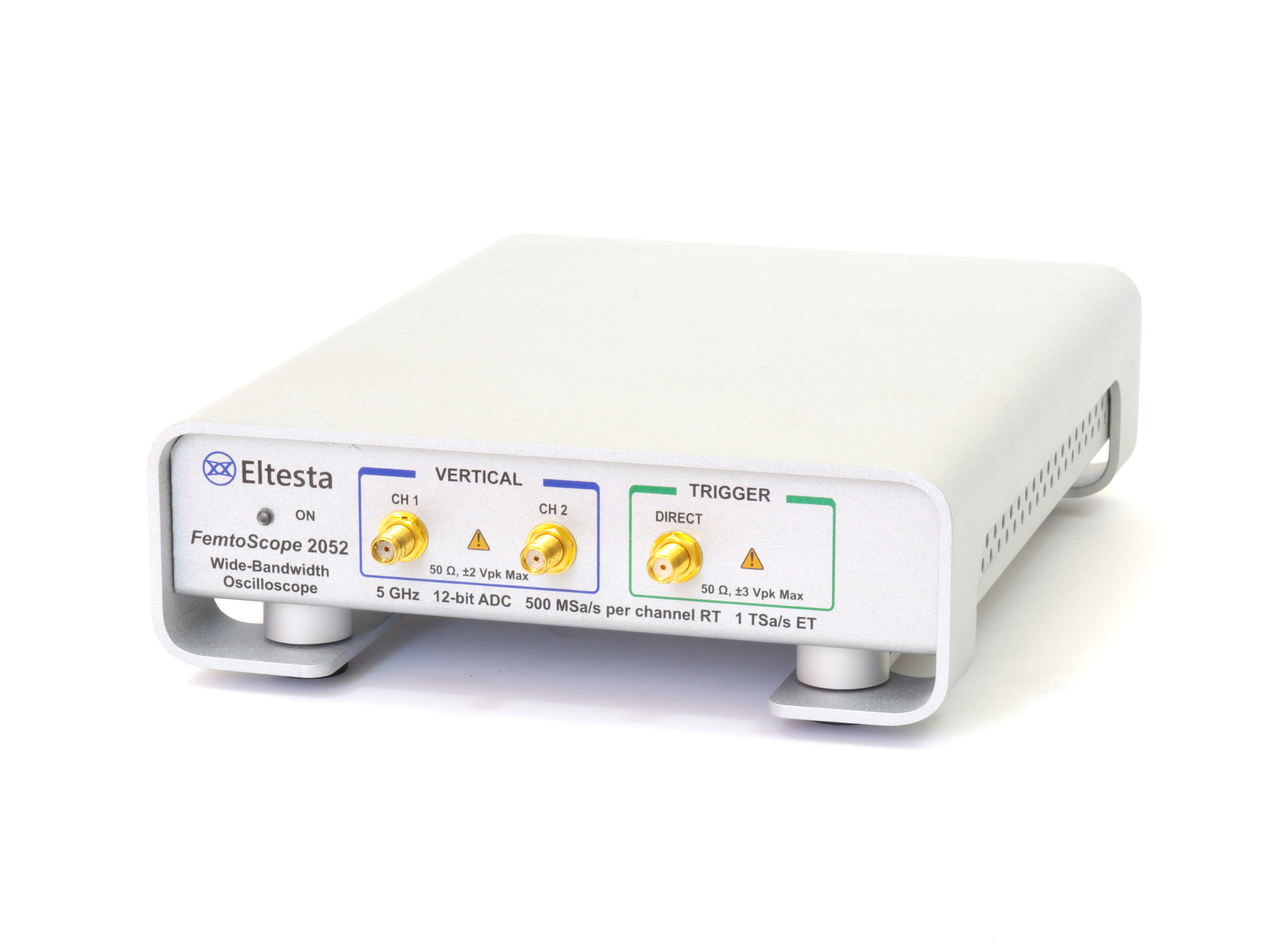
SONET/SDH (10)	OC1/STMO (51.84 Mb/s), OC3/STM1 (155.52 Mb/s), OC9/STM3 (466.56 Mb/s), OC12/STM4 (622.08 Mb/s), OC18/STM6 (933.12 Mb/s), OC24/STM8 (1.2442 Gb/s), OC48/STM16 (2.48832 Gb/s), FEC 2666 (2.6666 Gb/s)
		OC192/STM64 (9.95328 Gb/s), FEC1066 (10.664 Gb/s)
Fibre Channel (31)	FC133 Electrical (132.8 Mb/s), FC133 Optical (132.8 Mb/s), FC266 Electrical (265.6 Mb/s), FC266 Optical (265.6 Mb/s), FC531 Electrical (531.35 Mb/s), FC531 Optical (531.35 Mb/s), FC1063 Electrical (1.0625 Gb/s), FC1063 Optical (1.0625 Gb/s), FC1063 Optical PI Rev13 (1.0625 Gb/s), FC1063E Abs Beta Rx.mask (1.0625 Gb/s), FC1063E Abs Beta Tx.mask (1.0625 Gb/s), FC1063E Abs Delta Rx.mask (1.0625 Gb/s), FC1063E Abs Delta Tx.mask (1.0625 Gb/s), FC1063E Abs Gamma Rx.mask (1.0625 Gb/s), FC1063E Abs Gamma Tx.mask (1.0625 Gb/s), FC2125 Optical (2.1231 Gb/s), FC2125 Optical PI Rev13 (2.1231 Gb/s), FC2125E Abs Beta Rx.mask (2.125 Gb/s), FC2125E Abs Beta Tx.mask (2.125 Gb/s), FC2125E Abs Delta Rx.mask (2.125 Gb/s), FC2125E Abs Delta Tx.mask (2.125 Gb/s), FC2125E Abs Gamma Rx.mask (2.125 Gb/s), FC2125E Abs Gamma Tx.mask (2.125 Gb/s).
		FC4250 Optical PI Rev13 (4.25 Gb/s), FC4250E Abs Beta Rx.mask (4.25 Gb/s), FC4250E Abs Beta Tx.mask (4.25 Gb/s), FC4250E Abs Delta Rx.mask (4.25 Gb/s), FC4250E Abs Delta Tx.mask (4.25 Gb/s), FC4250E Abs Gamma Rx.mask (4.25 Gb/s), FC4250E Abs Gamma Tx.mask (4.25 Gb/s)
Ethernet (11)	100BASE-BX10 (125 Mb/s), 100BASE-BX/LX10 (125 Mb/s), 1.25 Gb/s 1000Base-CX Absolute TP2 (1.25 Gb/s), 1.25 Gb/s 1000Base-CX Absolute TP3 (1.25 Gb/s), GB Ethernet (1.25 Gb/s), 2XGB Ethernet (2.5 Gb/s), 3.125 Gb/s 10GBase-CX4 Absolute TP2 (3.125 Gb/s).
		10Gb Ethernet (9.953 Gb/s), 10GbE 9.953 (9.953 Gb/s), 10Gb Ethernet (10.3125 Gb/s), 10GbE 10.3125 (10.3125 Gb/s).
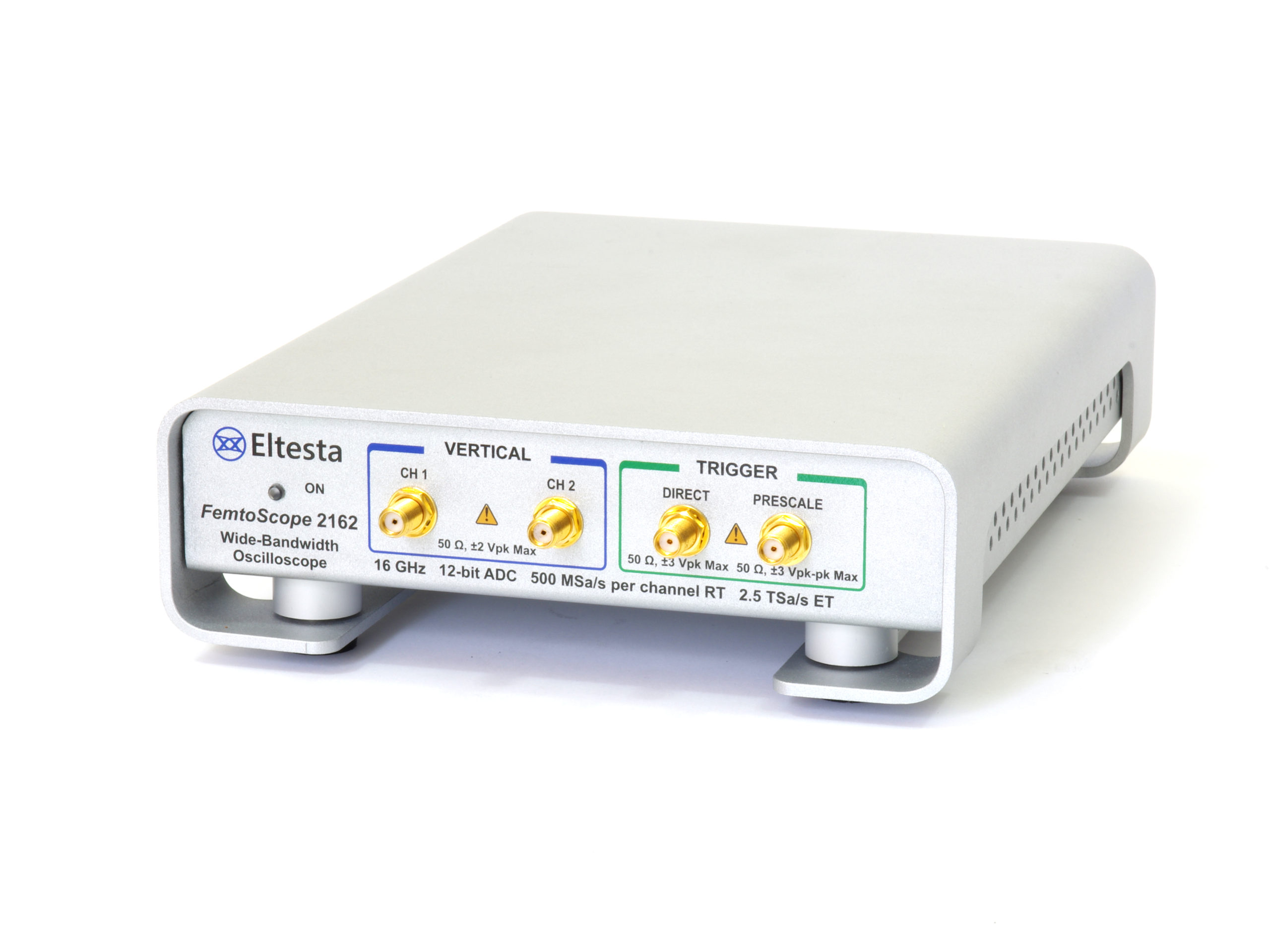
Infiniband (16)	2.5G InfiniBand Cable mask (2.5 Gb/s), 2.5G InfiniBand Driver Test Point 1 (2.5 Gb/s), 2.5G InfiniBand Driver Test Point 10 (2.5 Gb/s), 2.5G InfiniBand Driver Test Point 2 (2.5 Gb/s), 2.5G InfiniBand Driver Test Point 3 (2.5 Gb/s), 2.5G InfiniBand Driver Test Point 4 (2.5 Gb/s), 2.5G InfiniBand Driver Test Point 5 (2.5 Gb/s), 2.5G InfiniBand Driver Test Point 6 (2.5 Gb/s), 2.5G InfiniBand Driver Test Point 7 (2.5 Gb/s), 2.5G InfiniBand Driver Test Point 8 (2.5 Gb/s), 2.5G InfiniBand Driver Test Point 9 (2.5 Gb/s), 2.5G InfiniBand Receiver mask (2.5 Gb/s), InfiniBand (2.5 Gb/s).
		5.0G InfiniBand Driver Test Point 1 (5 Gb/s), 5.0G InfiniBand Driver Test Point 6 (5 Gb/s), 5.0G InfiniBand Transmitter Pins (5 Gb/s)
XAUI (4)	3.125 Gb/s XAUI Far End (3.125 Gb/s), 3.125 Gb/s XAUI Far End (3.125 Gb/s), XAUI-E Far (3.125 Gb/s), XAUI-E Near (3.125 Gb/s)
ITU G.703 (14)	DS1, 100 Ω twisted pair (1.544 Mb/s), 2 Mb 120, 120 Ω twisted pair (2.048 Mb/s), 2 Mb 75, 75 Ω coax (2.048 Mb/s), DS2 110, 110 Ω twisted pair (6.312 Mb/s), DS2 75, 75 Ω coax (6.312 Mb/s), 8 Mb, 75 Ω coax (8.448 Mb/s), 34 Mb, 75 Ω coax (34.368 Mb/s), DS3, 75 Ω coax (44.736 Mb/s), 140 Mb 0, 75 Ω coax (139.264 Mb/s), 140 Mb 1, 75 Ω coax (139.264 Mb/s), 140 Mb 1 Inv, 75 Ω coax (139.264 Mb/s), 155 Mb 0, 75 Ω coax (155.520 Mb/s), 155 Mb 1, 75 Ω coax (155.520 Mb/s), 155 Mb 1 Inv, 75 Ω coax (155.520 Mb/s).
ANSI T1/102 (7)	DS1, 100 Ω twisted pair, (1.544 Mb/s), DS1C, 100 Ω twisted pair, (3.152 Mb/s), DS2, 110 Ω twisted pair, (6.312 Mb/s), DS3, 75 Ω coax, (44.736 Mb/s), STS1 Eye, 75 Ω coax, (51.84 Mb/s), STS1 Pulse, 75 Ω coax, (51.84 Mb/s), STS3, 75 Ω coax, (155.520 Mb/s)
RapidIO (9)	RapidIO Serial Level 1, 1.25G Rx (1.25 Gb/s), RapidIO Serial Level 1, 1.25G Tx LR (1.25 Gb/s), RapidIO Serial Level 1, 1.25G Tx SR (1.25 Gb/s), RapidIO Serial Level 1, 2.5G Rx (2.5 Gb/s), RapidIO Serial Level 1, 2.5G Tx LR (2.5 Gb/s), RapidIO Serial Level 1, 2.5G Tx SR (2.5 Gb/s), RapidIO Serial Level 1, 3.125G Rx (3.125 Gb/s), RapidIO Serial Level 1, 3.125G Tx LR (3.125 Gb/s), RapidIO Serial Level 1, 3.125G Tx SR (3.125Gb/s)
PCI Express (41)	R1.0a 2.5G Add-in Card Transmitter Non-Transition bit mask (2.5 Gb/s), R1.0a 2.5G Add-in Card Transmitter Transition bit mask (2.5 Gb/s), R1.0a 2.5G Exp.Card Host Non-Transition bit mask (2.5 Gb/s), R1.0a 2.5G Exp.Card Host Transition bit mask (2.5 Gb/s), R1.0a 2.5G Exp.Card Module Non-Transition bit mask (2.5 Gb/s), R1.0a 2.5G Exp.Card Module Transition bit mask (2.5 Gb/s), R1.0a 2.5G Exp.Card Transmitter Non-Transition bit mask (2.5 Gb/s), R1.0a 2.5G Exp.Card Transmitter Transition bit mask (2.5 Gb/s), R1.1 2.5G Add-in Card Transmitter Non-Transition bit mask (2.5 Gb/s), R1.1 2.5G Add-in Card Transmitter Transition bit mask (2.5 Gb/s), R1.1 2.5G Cable Receiver End Non-Transition bit mask (2.5 Gb/s), R1.1 2.5G Cable Receiver End Transition bit mask (2.5 Gb/s), R1.1 2.5G Cable Transmitter End Non-Transition bit mask (2.5 Gb/s), R1.1 2.5G Cable Transmitter End Transition bit mask (2.5 Gb/s), R1.1 2.5G Express Module System Non-Transition bit mask (2.5 Gb/s), R1.1 2.5G Express Module System Transition bit mask (2.5 Gb/s), R1.1 2.5G Express Module Transmitter Path Non-Transition bit mask (2.5 Gb/s), R1.1 2.5G Express Module Transmitter Path Transition bit mask (2.5 Gb/s), R1.1 2.5G Receiver mask (2.5 Gb/s), R1.1 2.5G System Board Transmitter Non-Transition bit mask (2.5 Gb/s), R1.1 2.5G System Board Transmitter Transition bit mask (2.5 Gb/s), R1.1 2.5G Transmitter Non-Transition bit mask (2.5 Gb/s), R1.1 2.5G Transmitter Transition bit mask (2.5 Gb/s)
		R2.0 5.0G Add-in Card 35 dB Transmitter Non-Transition bit mask (5 Gb/s), R2.0 5.0G Add-in Card 60 dB Transmitter Non-Transition bit mask (5 Gb/s), 2.0 5.0G Add-in Card 35 dB Transmitter Transition bit mask (5 Gb/s), R2.0 5.0G Add-in Card 60 dB Transmitter Transition bit mask (5 Gb/s), R2.0 5.0G Mobile Transmitter mask (5 Gb/s), R2.0 5.0G Receiver mask (5 Gb/s), R2.0 5.0G System Board Transmitter Non-Transition bit mask (5 Gb/s), R2.0 5.0G System Board Transmitter Transition bit mask (5 Gb/s), R2.0 5.0G Transmitter Non-Transition bit mask (5 Gb/s), R2.0 5.0G Transmitter Transition bit mask (5 Gb/s). R2.1 5.0G Transmitter Non-Transition bit mask (5 Gb/s), R2.1 5.0G Transmitter Transition bit mask (5 Gb/s)
Serial ATA (24)	Ext Length, 1.5G 250 Cycle, Rx Mask (1.5 Gb/s), Ext Length, 1.5G 250 Cycle, Tx Mask (1.5 Gb/s), Ext Length, 1.5G 5 Cycle, Rx Mask (1.5 Gb/s), Ext Length, 1.5G 5 Cycle, Tx Mask (1.5 Gb/s), Gen1, 1.5G 250 Cycle, Rx Mask (1.5 Gb/s), Gen1, 1.5G 250 Cycle, Tx Mask (1.5 Gb/s), Gen1, 1.5G 5 Cycle, Rx Mask (1.5 Gb/s), Gen1, 1.5G 5 Cycle, Tx Mask (1.5 Gb/s), Gen1m, 1.5G 250 Cycle, Rx Mask (1.5 Gb/s), Gen1m, 1.5G 250 Cycle, Tx Mask (1.5 Gb/s), Gen1m, 1.5G 5 Cycle, Rx Mask (1.5 Gb/s), Gen1m, 1.5G 5 Cycle, Tx Mask (1.5 Gb/s), Ext Length, 3.0G 250 Cycle, Rx Mask (3 Gb/s), Ext Length, 3.0G 250 Cycle, Tx Mask (3 Gb/s), Ext Length, 3.0G 5 Cycle, Rx Mask (3 Gb/s), Ext Length, 3.0G 5 Cycle, Tx Mask (3 Gb/s), Gen1, 3.0G 250 Cycle, Rx Mask (3 Gb/s), Gen1, 3.0G 250 Cycle, Tx Mask (3 Gb/s), Gen1, 3.0G 5 Cycle, Rx Mask (3 Gb/s), Gen1, 3.0G 5 Cycle, Tx Mask (3 Gb/s), Gen1m, 3.0G 250 Cycle, Rx Mask (3 Gb/s), Gen1m, 3.0G 250 Cycle, Tx Mask (3 Gb/s), Gen1m, 3.0G 5 Cycle, Rx Mask (3 Gb/s), Gen1m, 3.0G 5 Cycle, Tx Mask (3 Gb/s).
Mask margin	Available for industry-standard mask testing
Automask creation	Masks are created automatically for single-valued voltage signals. Automask specifies both delta X and delta Y tolerances. The failure actions are identical to those of limit testing.
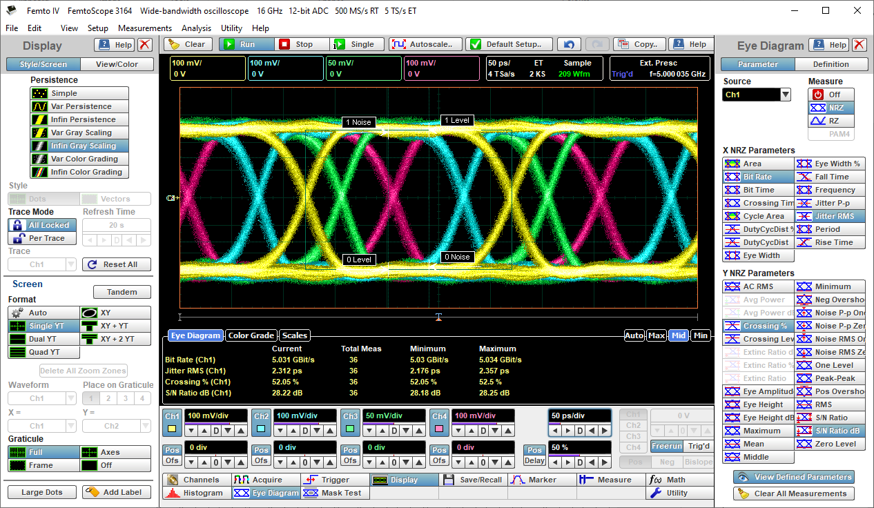
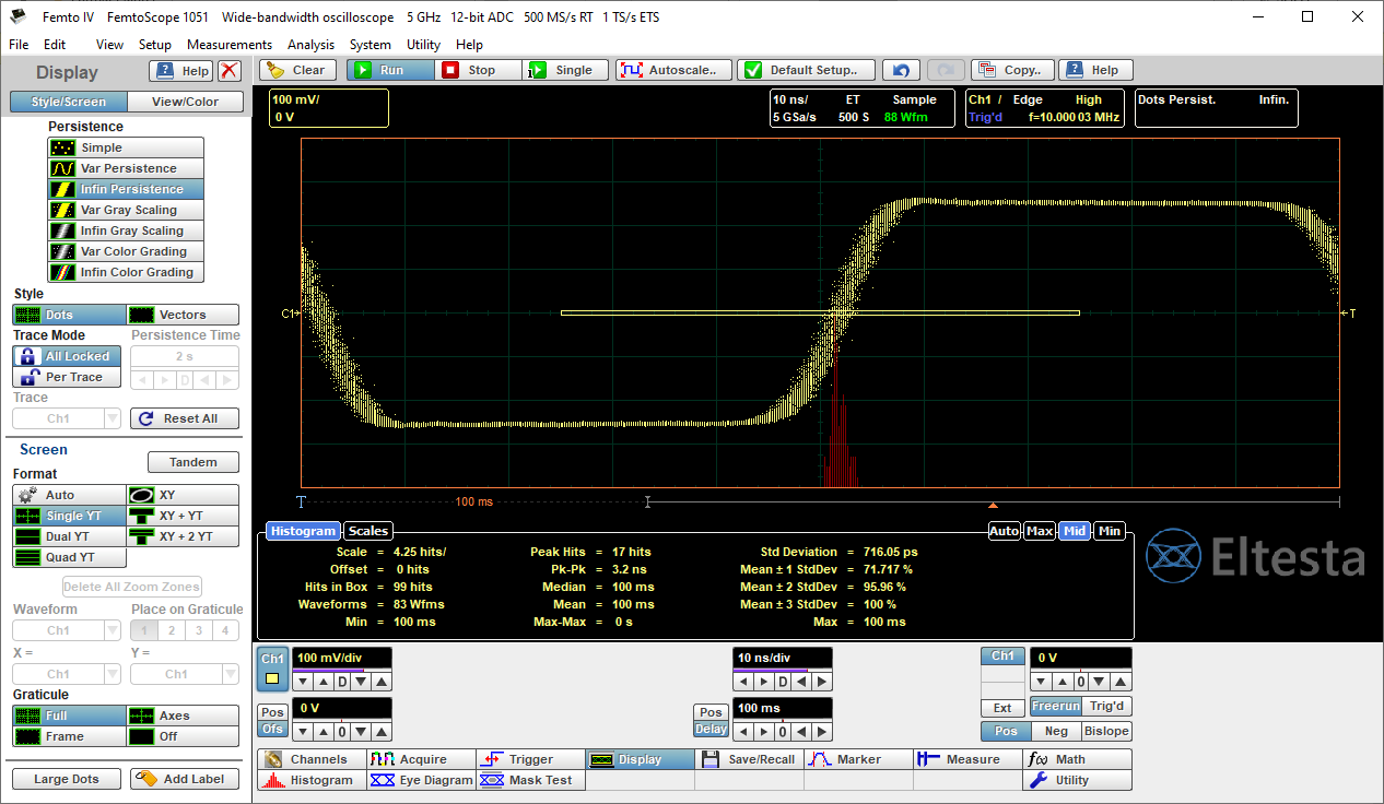
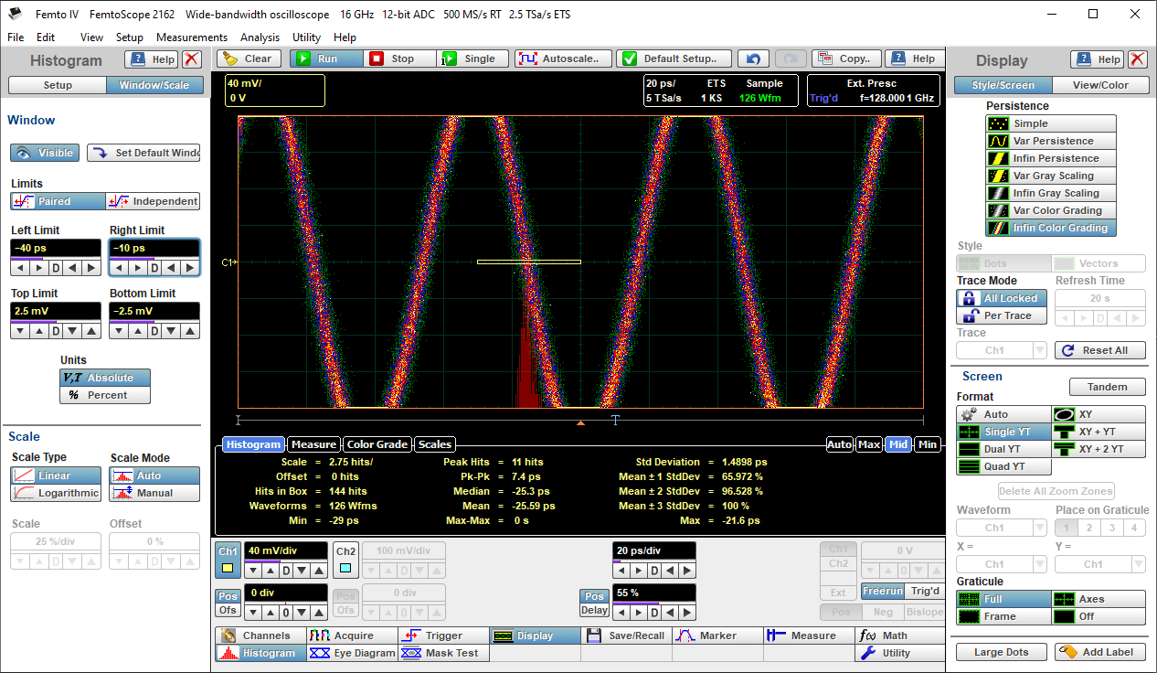
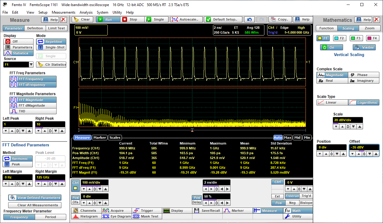
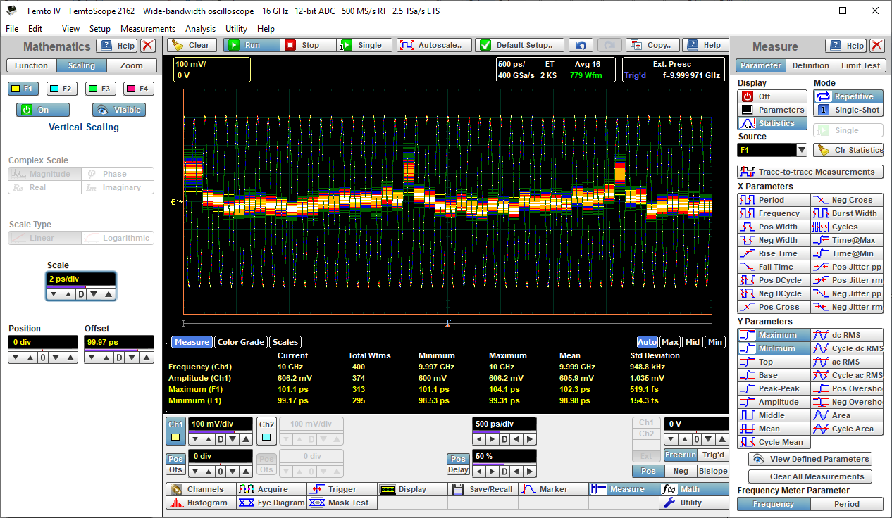
Data collected during test	Total number of waveforms examined, number of failed samples, number of hits within each polygon boundary

System requirements	FS1051	FS3054	FS1161	FS3164
Processor	Pentium-class processor or equivalent
Memory	4 GB
Disk space	Software occupies about 50 MB
Operating system	Windows 7, Windows 8 or Windows 10. 32‑bit and 64‑bit versions
PC connection port
USB	USB 2.0 (high speed). Also compatible with USB 3.0
LAN	N/A	LAN	N/A	LAN

Calibrator Output	FemtoScope 3000 only
Output mode	DC, 1 kHz square, Meander with frequency from 15.266 Hz to 500 kHz.
Output DC level	Adjustable from –1 V to +1 V into 50 Ω. Coarse increment: 50 mV, fine increment: 1 mV.
Output DC level accuracy	± 1 mV ± 0.5% of output DC level
Output impedance	50 Ω nominal
Rise/Fall time	150 ns, typical
Output connectors	SMA female

Trigger Output	FemtoScope 1000	FemtoScope 3000
Timing	Positive transition equivalent to acquisition trigger point.
Low level	(–0.2 ± 0.1) V. Measured into 50 Ω.
Amplitude	(900 ± 200) mV. Measured into 50 Ω.
Rise time	10% to 90%: ≤ 0.45 ns. 20% to 80%: ≤ 0.3 ns.
RMS jitter	2 ps or less.
Output delay	(4 ± 1) ns
Output coupling	DC-coupled
Output connectors	SMA female

Recovered Data Output	FemtoScope 2052	FemtoScope 2162
Data Rate	6.5 Mb/s to 5 Gb/s	6.5 Mb/s to 11.3 Gb/s
Eye amplitude	250 mV p-p typical
Eye rise/fall time	20%–80%: 70 ps, typical. Measured at 5-GHz channel.	20%–80%: 50 ps, typical. Measured at 16-GHz channel
RMS jitter	2 ps +1% of UI, typical
Output coupling	AC-coupled
Output connections	SMA female

Recovered Clock Output	FemtoScope 2052	FemtoScope 2162
Output frequency	Half rate clock output, 3.25 MHz to 2.5 GHz	Half rate clock output, 3.25 MHz to 5.65 GHz
Output amplitude	250 mV p-p, typical
Output coupling	AC-coupled
Output connectors	SMA female

System requirements	FemtoScope 1000	FemtoScope 2000	FemtoScope 3000
Power requirements
Power supply voltage	+12 V ± 5%
Power supply current	1.3 A max	1.8 A max	2.7 A max
Protection	Auto shutdown on excess or reverse voltage
AC-DC adaptor	Universal adaptor supplied
Physical characteristics
Dimensions
Width	113.9 mm	160 mm	244 mm
Height	33.5 mm w/o feet, 41.8 mm with feet	50 mm w/o feet, 54 mm with feet	64 mm
Depth	162 mm (w/o connectors), 187 mm (with connectors)	210 mm (w/o connectors), 225 mm (with connectors)	233 mm
Net weight	370 g	790 g	1.52 kg
Environmental conditions
Temperature	Normal: +5°C to +40°C. For quoted accuracy: +15°C to +25°C. Storage: –20°C to +50°C.
Humidity	Operating: Up to 85 % relative humidity at +25°C. Storage: Up to 95 % relative humidity

Models

Discover out models range

	FS1051	FS1161	FS2052	FS2162	FS3054	FS3164
CDR
Prescaled Trigger
Accessories included
Price	€6 490	€8 990	€8 990	€15 490	€11 990	€20 490
Buy now
	FS1051	FS1161	FS2052	FS2162	FS3054	FS3164